Chapter 8 : Machine Learning
In this chapter, we will cover the following topics:
- 8.1. Getting started with scikit-learn
- 8.2. Predicting who will survive on the Titanic with logistic regression *
- 8.3. Learning to recognize handwritten digits with a K-nearest neighbors classifier
- 8.4. Learning from text — Naive Bayes for Natural Language Processing
- 8.5. Using support vector machines for classification tasks
- 8.6. Using a random forest to select important features for regression
- 8.7. Reducing the dimensionality of a dataset with a principal component analysis *
- 8.8. Detecting hidden structures in a dataset with clustering
In the previous chapter, we were interested in getting insight into data, understanding complex phenomena through partial observations, and making informed decisions in the presence of uncertainty. Here, we are still interested in analyzing and processing data using statistical tools. However, the goal is not necessarily to understand the data, but to learn from it.
Learning from data is close to what we do as humans. From our experience, we intuitively learn general facts and relations about the world, even if we don't fully understand their complexity. The increasing computational power of computers makes them able to learn from data too. That's the heart of machine learning, a branch of artificial intelligence at the intersection of computer science, statistics, and applied mathematics.
This chapter is a hands-on introduction to some of the most basic methods in machine learning. These methods are routinely used by data scientists. We will use these methods with scikit-learn, a popular and user-friendly Python package for machine learning.
A bit of vocabulary
In this introduction, we will explain the fundamental definitions and concepts of machine learning.
Learning from data
In machine learning, most data can be represented as a table of numerical values. Every row is called an observation, a sample, or a data point. Every column is called a feature or a variable.
Let's call \(N\) the number of rows (or the number of points) and \(D\) the number of columns (or number of features). The number \(D\) is also called the dimensionality of the data. The reason is that we can view this table as a set \(E\) of vectors in a space with \(D\) dimensions (or vector space). Here, a vector \(x\) contains \(D\) numbers \((x_1, ..., x_D)\), also called components. This mathematical point of view is very useful and we will use it throughout this chapter.
We make the distinction between supervised learning and unsupervised learning:
- Supervised learning is when we have a label \(y\) associated with a data point \(x\). The goal is to learn the mapping from \(x\) to \(y\) from our data. The data gives us this mapping for a finite set of points, but what we want is to generalize this mapping to the full set \(E\), or at least to a larger set of points.
- Unsupervised learning is when we don't have any labels. What we want to do is discover some form of hidden structure in the data.
Supervised learning
Mathematically, supervised learning consists of finding a function \(f\) that maps the set of points \(E\) to a set of labels \(F\), knowing a finite set of associations \((x, y)\), which is given by our data. This is what generalization is about: after observing the pairs \((x_i, y_i)\), given a new \(x\), we are able to find the corresponding \(y\) by applying the function \(f\) to \(x\).
It is a common practice to split the set of data points into two subsets: the training set and the test set. We learn the function \(f\) on the training set and test it on the test set. This is essential when assessing the predictive power of a model. By training and testing a model on the same set, our model might not be able to generalize well. This is the fundamental concept of overfitting, which we will detail later in this chapter.
We generally make the distinction between classification and regression, two particular instances of supervised learning.
Classification is when our labels \(y\) can only take a finite set of values (categories). Examples include:
- Handwritten digit recognition: \(x\) is an image with a handwritten digit; \(y\) is a digit between 0 and 9
- Spam filtering: \(x\) is an e-mail and \(y\) is 1 or 0, depending on whether that e-mail is spam or not
Regression is when our labels \(y\) can take any real (continuous) value. Examples include:
- Predicting stock market data
- Predicting sales
- Detecting the age of a person from a picture
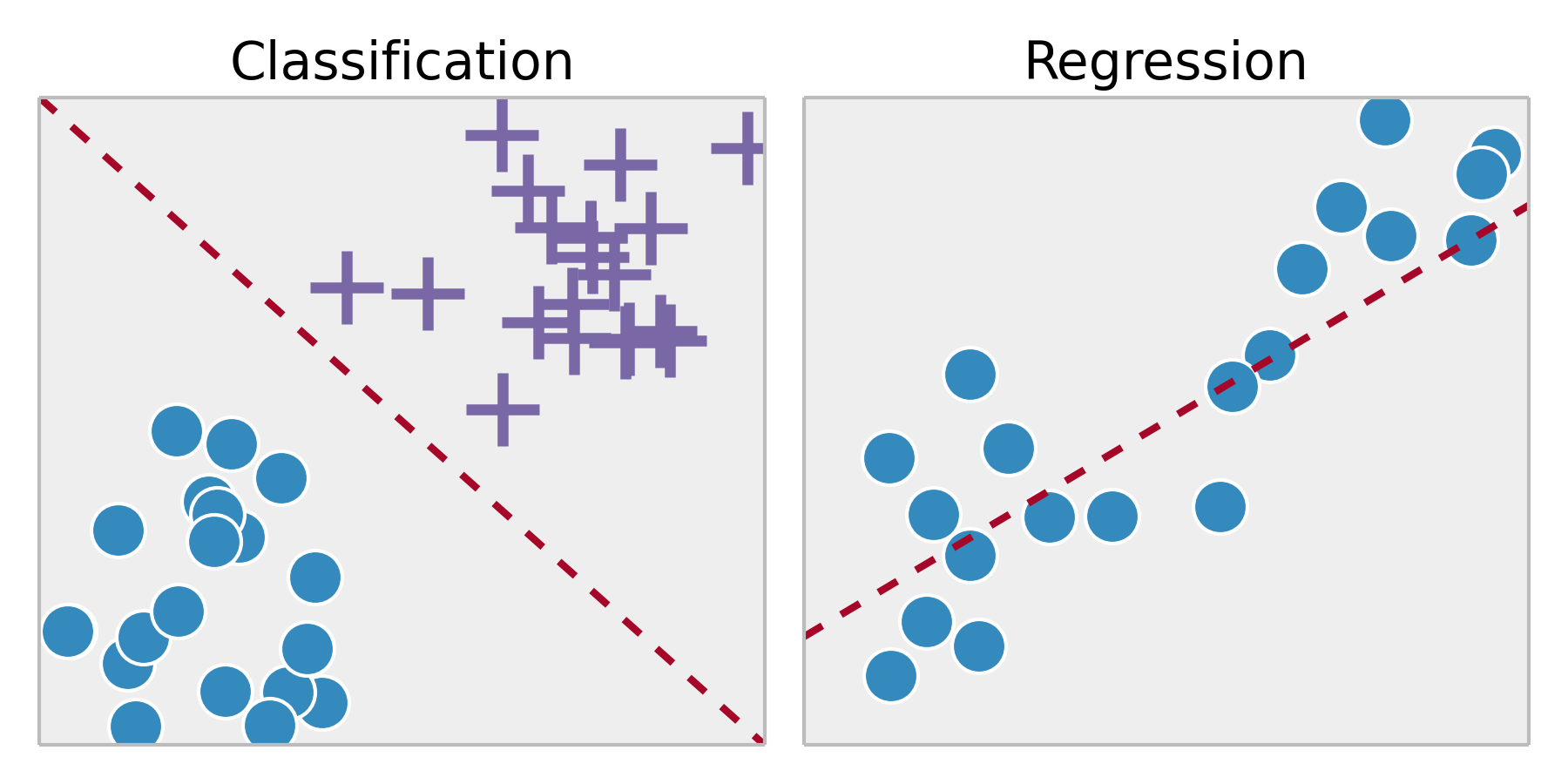
A classification task yields a division of our space \(E\) in different regions (also called partitions), each region being associated to one particular value of the label \(y\). A regression task yields a mathematical model that associates a real number to any point \(x\) in the space \(E\). This difference is illustrated in the following figure:
Classification and regression can be combined. For example, in the probit model, although the dependent variable is binary (classification), the probability that this variable belongs to one category can also be modeled (regression). We will see an example in the recipe about logistic regression. For more information on the probit model, refer to https://en.wikipedia.org/wiki/Probit_model.
Unsupervised learning
Broadly speaking, unsupervised learning helps us discover systemic structures in our data. This is harder to grasp than supervised learning, in that there is generally no precise question and answer.
Here are a few important tasks related to unsupervised learning:
- Clustering: Grouping similar points together within clusters
- Density estimation: Estimating a probability density function that can explain the distribution of the data points
- Dimension reduction: Getting a simple representation of high-dimensional data points by projecting them onto a lower-dimensional space (notably for data visualization)
- Manifold learning: Finding a low-dimensional manifold containing the data points (also known as nonlinear dimension reduction)
Feature selection and feature extraction
In a supervised learning context, when our data contains many features, it is sometimes necessary to choose a subset of them. The features we want to keep are those that are most relevant to our question. This is the problem of feature selection.
Additionally, we might want to extract new features by applying complex transformations on our original dataset. This is feature extraction. For example, in computer vision, training a classifier directly on the pixels is not the most efficient method in general. We might want to extract the relevant points of interest or make appropriate mathematical transformations. These steps depend on our dataset and on the questions we want to answer.
For example, it is often necessary to preprocess the data before learning models. Feature scaling (or data normalization) is a common preprocessing step where features are linearly rescaled to fit in the range \([-1,1]\) or \([0,1]\).
Feature extraction and feature selection involve a balanced combination of domain expertise, intuition, and mathematical methods. These early steps are crucial, and they might be even more important than the learning steps themselves. The reason is that the few dimensions that are relevant to our problem are generally hidden in the high dimensionality of our dataset. We need to uncover the low-dimensional structure of interest to improve the efficiency of the learning models.
We will see a few feature selection and feature extraction methods in this chapter. Methods that are specific to signals, images, or sounds will be covered in Chapter 10, Signal Processing, and Chapter 11, Image and Audio Processing.
Deep learning has profoundly revolutionized machine learning in the last few years. A major characteristic of this range of methods is that feature selection and extraction are often included in the model itself. The most relevant features are automatically selected by the algorithm. This method works particularly well on images, sounds, and videos. Typically, however, deep learning requires a huge amount of training data and computational power. Covering deep learning methods in Python is beyond the scope of this book, but we give a few references at the end of this introduction.
Here are a few further references:
- Feature selection in scikit-learn, documented at http://scikit-learn.org/stable/modules/feature_selection.html
- Feature selection on Wikipedia at https://en.wikipedia.org/wiki/Feature_selection
Overfitting, underfitting, and the bias-variance tradeoff
A central notion in machine learning is the trade-off between overfitting and underfitting. A model may be able to represent our data accurately. However, if it is too accurate, it might not generalize well to unobserved data. For example, in facial recognition, a too-accurate model would be unable to identify someone who styled their hair differently that day. The reason is that our model might learn irrelevant features in the training data. On the contrary, an insufficiently trained model would not generalize well either. For example, it would be unable to correctly recognize twins. For more information on overfitting, refer to https://en.wikipedia.org/wiki/Overfitting.
A popular solution to reduce overfitting consists of adding structure to the model, for example, with regularization. This method favors simpler models during training (Occam's razor). You will find more information at https://en.wikipedia.org/wiki/Regularization_%28mathematics%29.
The bias-variance dilemma is closely related to the issue of overfitting and underfitting. The bias of a model quantifies how precise it is across training sets. The variance quantifies how sensitive the model is to small changes in the training set. A robust model is not overly sensitive to small changes. The dilemma involves minimizing both bias and variance; we want a precise and robust model. Simpler models tend to be less accurate but more robust. Complex models tend to be more accurate but less robust. For more information on the bias-variance dilemma, refer to https://en.wikipedia.org/wiki/Bias-variance_dilemma.
The importance of this trade-off cannot be overstated. This question pervades the entire discipline of machine learning. We will see concrete examples in this chapter.
Model selection
As we will see in this chapter, there are many supervised and unsupervised algorithms. For example, well-known classifiers that we will cover in this chapter include logistic regression, nearest-neighbors, Naive Bayes, and support vector machines. There are many other algorithms that we can't cover here.
No model performs uniformly better than the others. One model may perform well on one dataset and badly on another. This is the question of model selection.
We will see systematic methods to assess the quality of a model on a particular dataset (notably cross-validation). In practice, machine learning is not an "exact science" in that it frequently involves trial and error. We need to try different models and empirically choose the one that performs best.
That being said, understanding the details of the learning models allows us to gain intuition about which model is best adapted to our current problem.
Here are a few references on this question:
- Model selection on Wikipedia, available at https://en.wikipedia.org/wiki/Model_selection
- Model evaluation in scikit-learn's documentation, available at http://scikit-learn.org/stable/modules/model_evaluation.html
- Blog post on how to choose a classifier, available at http://blog.echen.me/2011/04/27/choosing-a-machine-learning-classifier/
Machine learning references
Here are a few excellent, math-heavy textbooks on machine learning:
- Pattern Recognition and Machine Learning, Christopher M. Bishop, (2006), Springer
- Machine Learning – A Probabilistic Perspective, Kevin P. Murphy, (2012), MIT Press
- The Elements of Statistical Learning, Trevor Hastie, Robert Tibshirani, Jerome Friedman, (2009), Springer
Here are a few books more oriented toward programmers without a strong mathematical background:
- Machine Learning for Hackers, Drew Conway, John Myles White, (2012), O'Reilly Media
- Machine Learning in Action, Peter Harrington, (2012), Manning Publications Co.
- Python Machine Learning, Sebastian Raschka (2015), Packt Publishing.
Further references can be found here:
- Awesome Machine Learning resources, at https://github.com/josephmisiti/awesome-machine-learning
- Statistical Learning lectures on Awesome Math, at https://github.com/rossant/awesome-math/#statistical-learning
Important classes of machine learning methods that we couldn't cover in this chapter include neural networks and deep learning. Deep learning is the subject of very active research in machine learning. Many state-of-the-art results are currently achieved by using deep learning methods.
Here are few references on deep learning:
- Awesome Deep Learning resources, at https://github.com/ChristosChristofidis/awesome-deep-learning
- Coursera Deep Learning course, at https://www.coursera.org/specializations/deep-learning
- Udacity Deep Learning course, at https://www.udacity.com/course/deep-learning--ud730
- Keras Tutorial: Deep Learning in Python, at https://www.datacamp.com/community/tutorials/deep-learning-python
- Deep learning with Python, a book by François Chollet, Manning Publications, at https://www.manning.com/books/deep-learning-with-python
Finally, here are a few lists of public datasets that can be used for data science projects:
- List of datasets for machine learning research, at https://en.wikipedia.org/wiki/List_of_datasets_for_machine_learning_research
- Awesome public datasets, at https://github.com/caesar0301/awesome-public-datasets
- Datasets for Data Science and Machine Learning at https://elitedatascience.com/datasets
- Kaggle Datasets, at https://www.kaggle.com/datasets