4.5. Understanding the internals of NumPy to avoid unnecessary array copying
 This is one of the 100+ free recipes of the IPython Cookbook, Second Edition, by Cyrille Rossant, a guide to numerical computing and data science in the Jupyter Notebook. The ebook and printed book are available for purchase at Packt Publishing.
▶ Text on GitHub with a CC-BY-NC-ND license
▶ Code on GitHub with a MIT license
▶ Go to Chapter 4 : Profiling and Optimization
▶ Get the Jupyter notebook
We can achieve significant performance speedups with NumPy over native Python code, particularly when our computations follow the Single Instruction, Multiple Data (SIMD) paradigm. However, it is also possible to unintentionally write non-optimized code with NumPy.
In the next few recipes, we will see some tricks that can help us write optimized NumPy code. In this recipe, we will see how to avoid unnecessary array copies in order to save memory. In that respect, we will need to dig into the internals of NumPy.
Getting ready
First, we need a way to check whether two arrays share the same underlying data buffer in memory. Let's define a function aid() that returns the memory location of the underlying data buffer:
import numpy as np
def aid(x):
    # This function returns the memory
    # block address of an array.
    return x.__array_interface__['data'][0]
Two arrays with the same data location (as returned by aid()) share the same underlying data buffer. However, the opposite is true only if the arrays have the same offset (meaning that they have the same first element). Two shared arrays with different offsets will have slightly different memory locations, as shown in the following example:
a = np.zeros(3)
aid(a), aid(a[1:])
(21535472, 21535480)
In the next few recipes, we'll make sure to use this method with arrays that have the same offset. Here is a more general and reliable solution for finding out whether two arrays share the same data:
def get_data_base(arr):
    """For a given NumPy array, find the base array
    that owns the actual data."""
    base = arr
    while isinstance(base.base, np.ndarray):
        base = base.base
    return base


def arrays_share_data(x, y):
    return get_data_base(x) is get_data_base(y)
print(arrays_share_data(a, a.copy()))
False
print(arrays_share_data(a, a[:1]))
True
Thanks to Michael Droettboom for pointing this out and proposing this alternative solution.
How to do it...
Computations with NumPy arrays may involve internal copies between blocks of memory. These copies are not always necessary, in which case they should be avoided, as we will see in the following tips.
1. We may sometimes need to make a copy of an array; for instance, if we need to manipulate an array while keeping an original copy in memory:
import numpy as np
a = np.zeros(10)
ax = aid(a)
ax
32250112
b = a.copy()
aid(b) == ax
False
2. Array computations can involve in-place operations (the first example in the following code: the array is modified) or implicit-copy operations (the second example: a new array is created):
a *= 2
aid(a) == ax
True
c = a * 2
aid(c) == ax
False
Implicit-copy operations are slower, as shown here:
%%timeit a = np.zeros(10000000)
a *= 2
4.85 ms ± 24 µs per loop (mean ± std. dev. of 7 runs,
100 loops each)
%%timeit a = np.zeros(10000000)
b = a * 2
7.7 ms ± 105 µs per loop (mean ± std. dev. of 7 runs,
100 loops each)
3. Reshaping an array may or may not involve a copy. The reasons will be explained in the How it works... section. For instance, reshaping a 2D matrix does not involve a copy, unless it is transposed (or more generally, non-contiguous):
a = np.zeros((100, 100))
ax = aid(a)
b = a.reshape((1, -1))
aid(b) == ax
True
c = a.T.reshape((1, -1))
aid(c) == ax
False
Therefore, the latter instruction is significantly slower than the former:
%timeit b = a.reshape((1, -1))
330 ns ± 0.517 ns per loop (mean ± std. dev. of 7 runs
    1000000 loops each)
%timeit a.T.reshape((1, -1))
5 µs ± 5.68 ns per loop (mean ± std. dev. of 7 runs,
    100000 loops each)
4. Both the flatten() and the ravel() methods of an array reshape it into a 1D vector (a flattened array). However, the flatten() method always returns a copy, and the ravel() method returns a copy only if necessary (thus it's faster, especially with large arrays).
d = a.flatten()
aid(d) == ax
False
e = a.ravel()
aid(e) == ax
True
%timeit a.flatten()
2.3 µs ± 18.1 ns per loop (mean ± std. dev. of 7 runs,
100000 loops each)
%timeit a.ravel()
199 ns ± 5.02 ns per loop (mean ± std. dev. of 7 runs,
10000000 loops each)
5. Broadcasting rules allow us to make computations on arrays with different but compatible shapes. In other words, we don't always need to reshape or tile our arrays to make their shapes match. The following example illustrates two ways of doing an outer product between two vectors: the first method involves array tiling, the second one (faster) involves broadcasting:
n = 1000
a = np.arange(n)
ac = a[:, np.newaxis]  # column vector
ar = a[np.newaxis, :]  # row vector
%timeit np.tile(ac, (1, n)) * np.tile(ar, (n, 1))
5.7 ms ± 42.6 µs per loop (mean ± std. dev. of 7 runs,
100 loops each)
%timeit ar * ac
784 µs ± 2.39 µs per loop (mean ± std. dev. of 7 runs,
1000 loops each)
How it works...
In this section, we will see what happens under the hood when using NumPy, and how this knowledge allows us to understand the tricks given in this recipe.
Why are NumPy arrays efficient?
A NumPy array is basically described by metadata (notably the number of dimensions, the shape, and the data type) and the actual data. The data is stored in a homogeneous and contiguous block of memory, at a particular address in system memory (Random Access Memory, or RAM). This block of memory is called the data buffer. This is the main difference between an array and a pure Python structure, such as a list, where the items are scattered across the system memory. This aspect is the critical feature that makes NumPy arrays so efficient.
Why is this so important? Here are the main reasons:
- Computations on arrays can be written very efficiently in a low-level language such as C (and a large part of NumPy is actually written in C). Knowing the address of the memory block and the data type, it is just simple arithmetic to loop over all items, for example. There would be a significant overhead to do that in Python with a list.
- Spatial locality in memory access patterns results in performance gains notably due to the CPU cache. Indeed, the cache loads bytes in chunks from RAM to the CPU registers. Adjacent items are then loaded very efficiently (sequential locality, or locality of reference).
- Finally, the fact that items are stored contiguously in memory allows NumPy to take advantage of vectorized instructions of modern CPUs, such as Intel's SSE and AVX, AMD's XOP, and so on. For example, multiple consecutive floating point numbers can be loaded in 128, 256, or 512 bits registers for vectorized arithmetical computations implemented as CPU instructions.
Additionally, NumPy can be linked to highly optimized linear algebra libraries such as BLAS and LAPACK through ATLAS or the Intel Math Kernel Library (MKL). A few specific matrix computations may also be multithreaded, taking advantage of the power of modern multicore processors.
In conclusion, storing data in a contiguous block of memory ensures that the architecture of modern CPUs is used optimally, in terms of memory access patterns, CPU cache, and vectorized instructions.
What is the difference between in-place and implicit-copy operations?
Let's explain the example in step 2. An expression such as a *= 2 corresponds to an in-place operation, where all values of the array are multiplied by two. By contrast, a = a*2 means that a new array containing the values of a*2 is created, and the variable a now points to this new array. The old array becomes unreferenced and will be deleted by the garbage collector. No memory allocation happens in the first case, contrary to the second case.
More generally, expressions such as a[i:j] are views to parts of an array; they point to the memory buffer containing the data. Modifying them with in-place operations changes the original array.
Knowing this subtlety of NumPy can help you fix some bugs (where an array is implicitly and unintentionally modified because of an operation on a view), and optimize the speed and memory consumption of your code by reducing the number of unnecessary copies.
Why can't some arrays be reshaped without a copy?
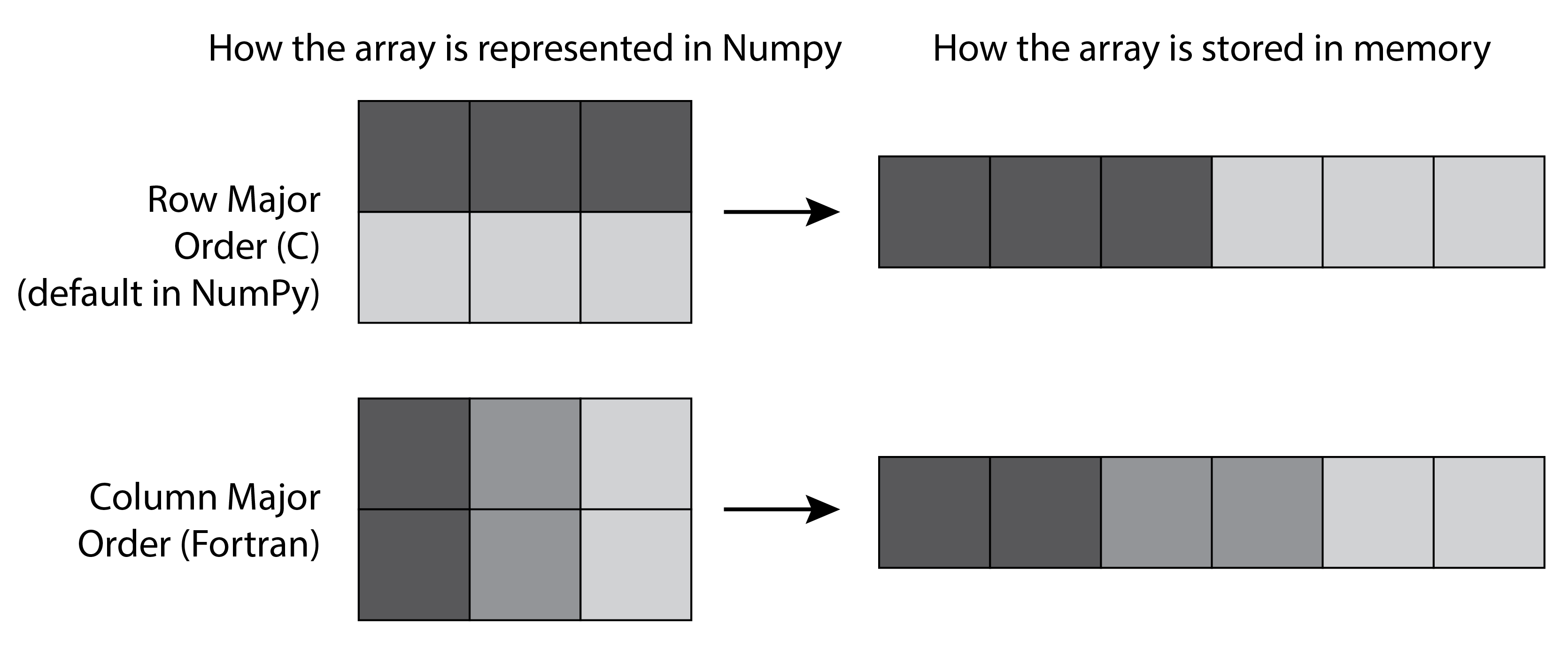
We explain the example in step 3 here, where a transposed 2D matrix cannot be flattened without a copy. A 2D matrix contains items indexed by two numbers (row and column), but it is stored internally as a 1D contiguous block of memory, accessible with a single number. There is more than one way of storing matrix items in a 1D block of memory: we can put the elements of the first row first, then the second row, and so on, or the elements of the first column first, then the second column, and so on. The first method is called row-major order, whereas the latter is called column-major order. Choosing between the two methods is only a matter of internal convention: NumPy uses the row-major order, like C, but unlike FORTRAN.

More generally, NumPy uses the notion of strides to convert between a multidimensional index and the memory location of the underlying (1D) sequence of elements. The specific mapping between array[i1, i2] and the relevant byte address of the internal data is given by:
offset = array.strides[0] * i1 + array.strides[1] * i2
When reshaping an array, NumPy avoids copies when possible by modifying the strides attribute. For example, when transposing a matrix, the order of strides is reversed, but the underlying data remains identical. However, flattening a transposed array cannot be accomplished simply by modifying strides, so a copy is needed.
Internal array layout can also explain some unexpected performance discrepancies between very similar NumPy operations. As a small exercise, can you explain the following benchmarks?
a = np.random.rand(5000, 5000)
%timeit a[0, :].sum()
2.91 µs ± 20 ns per loop (mean ± std. dev. of 7 runs,
    100000 loops each)
%timeit a[:, 0].sum()
33.7 µs ± 22.7 ns per loop (mean ± std. dev. of 7 runs
    10000 loops each)
What are NumPy broadcasting rules?
Broadcasting rules describe how arrays with different dimensions and/or shapes can be used for computations. The general rule is that two dimensions are compatible when they are equal, or when one of them is 1. NumPy uses this rule to compare the shapes of the two arrays element-wise, starting with the trailing dimensions and working its way forward. The smallest dimension is internally stretched to match the other dimension, but this operation does not involve any memory copy.
There's more...
Here are a few references:
- Broadcasting rules and examples, available at http://docs.scipy.org/doc/numpy/user/basics.broadcasting.html
- Array interface in NumPy, at http://docs.scipy.org/doc/numpy/reference/arrays.interface.html
- Locality of reference, at https://en.wikipedia.org/wiki/Locality_of_reference
- Internals of NumPy in the SciPy lectures notes, available at http://scipy-lectures.github.io/advanced/advanced_numpy/
- 100 NumPy exercises by Nicolas Rougier, available at http://www.loria.fr/~rougier/teaching/numpy.100/index.html
See also
- Using stride tricks with NumPy