12.2. Simulating an elementary cellular automaton
 This is one of the 100+ free recipes of the IPython Cookbook, Second Edition, by Cyrille Rossant, a guide to numerical computing and data science in the Jupyter Notebook. The ebook and printed book are available for purchase at Packt Publishing.
▶ Text on GitHub with a CC-BY-NC-ND license
▶ Code on GitHub with a MIT license
▶ Go to Chapter 12 : Deterministic Dynamical Systems
▶ Get the Jupyter notebook
Cellular automata are discrete dynamical systems evolving on a grid of cells. These cells can be in a finite number of states (for example, on/off). The evolution of a cellular automaton is governed by a set of rules, describing how the state of a cell changes according to the state of its neighbors.
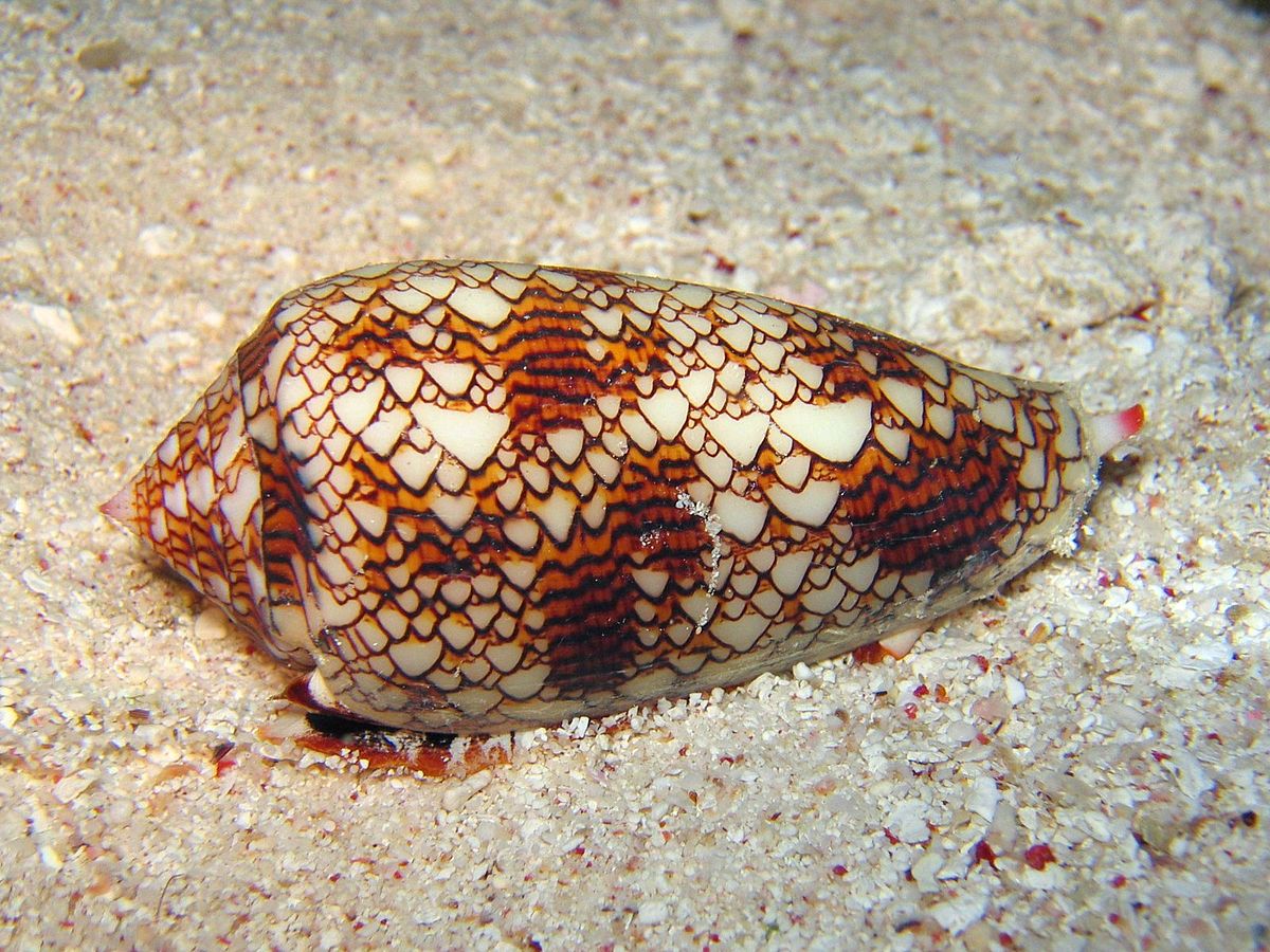
Although extremely simple, these models can initiate highly complex and chaotic behaviors. Cellular automata can model real-world phenomena such as car traffic, chemical reactions, propagation of fire in a forest, epidemic propagations, and much more. Cellular automata are also found in nature. For example, the patterns of some seashells are generated by natural cellular automata.
An elementary cellular automaton is a binary, one-dimensional automaton, where the rules concern the immediate left and right neighbors of every cell.
In this recipe, we will simulate elementary cellular automata with NumPy using their Wolfram code.
How to do it...
1. We import NumPy and matplotlib:
import numpy as np
import matplotlib.pyplot as plt
%matplotlib inline
2. We will use the following vector to obtain numbers written in binary representation:
u = np.array([[4], [2], [1]])
3. Let's write a function that performs an iteration on the grid, updating all cells at once according to the given rule in binary representation (we will give all explanations in the How it works... section). The first step consists of stacking circularly-shifted versions of the grid to get the LCR (left, center, right) triplets of each cell (y). Then, we convert these triplets into 3-bit numbers (z). Finally, we compute the next state of every cell using the specified rule:
def step(x, rule_b):
    """Compute a single stet of an elementary cellular
    automaton."""
    # The columns contains the L, C, R values
    # of all cells.
    y = np.vstack((np.roll(x, 1), x,
                   np.roll(x, -1))).astype(np.int8)
    # We get the LCR pattern numbers between 0 and 7.
    z = np.sum(y * u, axis=0).astype(np.int8)
    # We get the patterns given by the rule.
    return rule_b[7 - z]
4. We now write a function that simulates any elementary cellular automaton. First, we compute the binary representation of the rule (Wolfram Code). Then, we initialize the first row of the grid with random values. Finally, we apply the function step() iteratively on the grid:
def generate(rule, size=100, steps=100):
    """Simulate an elementary cellular automaton given
    its rule (number between 0 and 255)."""
    # Compute the binary representation of the rule.
    rule_b = np.array(
        [int(_) for _ in np.binary_repr(rule, 8)],
        dtype=np.int8)
    x = np.zeros((steps, size), dtype=np.int8)
    # Random initial state.
    x[0, :] = np.random.rand(size) < .5
    # Apply the step function iteratively.
    for i in range(steps - 1):
        x[i + 1, :] = step(x[i, :], rule_b)
    return x
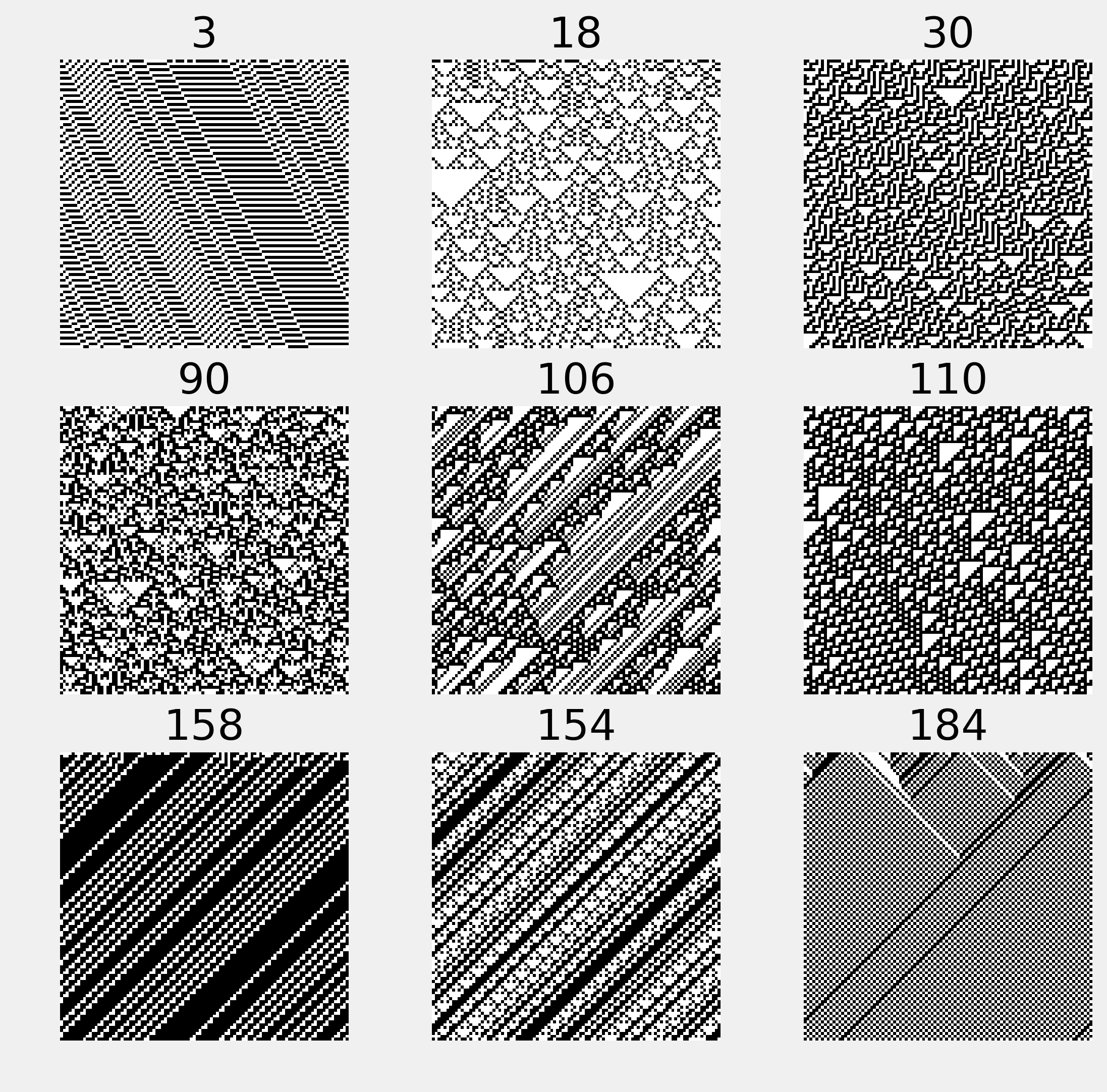
5. Now, we simulate and display nine different automata:
fig, axes = plt.subplots(3, 3, figsize=(8, 8))
rules = [3, 18, 30,
         90, 106, 110,
         158, 154, 184]
for ax, rule in zip(axes.flat, rules):
    x = generate(rule)
    ax.imshow(x, interpolation='none',
              cmap=plt.cm.binary)
    ax.set_axis_off()
    ax.set_title(str(rule))
How it works...
Let's consider an elementary cellular automaton in one dimension. Every cell \(C\) has two neighbors (\(L\) and \(R\)), and it can be either off (0) or on (1). Therefore, the future state of a cell depends on the current state of \(L\), \(C\), and \(R\). This triplet can be encoded as a number between 0 and 7 (three digits in binary representation).
A particular elementary cellular automaton is entirely determined by the outcome of each of these eight configurations. Therefore, there are 256 different elementary cellular automata (\(2^8\)). Each of these automata is identified by a number between 0 and 255.
We consider all eight LCR states in order: 111, 110, 101, ..., 001, 000. Each of the eight digits in the binary representation of the automaton's number corresponds to a LCR state (using the same order). For example, in the Rule 110 automaton (01101110 in binary representation), the state 111 yields a new state of 0 for the center cell, 110 yields 1, 101 yields 1, and so on. It has been shown that this particular automaton is Turing complete (or universal); it can theoretically simulate any computer program.
There's more...
Other types of cellular automata include Conway's Game of Life, in two dimensions. This famous system yields various dynamic patterns. It is also Turing complete.
Here are a few references:
- Cellular automata on Wikipedia, available at https://en.wikipedia.org/wiki/Cellular_automaton
- Elementary cellular automata on Wikipedia, available at https://en.wikipedia.org/wiki/Elementary_cellular_automaton
- Rule 110, described at https://en.wikipedia.org/wiki/Rule_110
- The Wolfram code, explained at https://en.wikipedia.org/wiki/Wolfram_code, assigns a 1D elementary cellular automaton to any number between 0 and 255
- Conway's Game of Life on Wikipedia, available at https://en.wikipedia.org/wiki/Conway's_Game_of_Life
- A computer implemented in Conway's Game of Life, at https://codegolf.stackexchange.com/questions/11880/build-a-working-game-of-tetris-in-conways-game-of-life