11.4. Finding points of interest in an image
 This is one of the 100+ free recipes of the IPython Cookbook, Second Edition, by Cyrille Rossant, a guide to numerical computing and data science in the Jupyter Notebook. The ebook and printed book are available for purchase at Packt Publishing.
▶ Text on GitHub with a CC-BY-NC-ND license
▶ Code on GitHub with a MIT license
▶ Go to Chapter 11 : Image and Audio Processing
▶ Get the Jupyter notebook
In an image, points of interest are positions where there might be edges, corners, or interesting objects. For example, in a landscape picture, points of interest can be located near a house or a person. Detecting points of interest is useful in image recognition, computer vision, or medical imaging.
In this recipe, we will find points of interest in an image with scikit-image. This will allow us to crop an image around the subject of the picture, even when this subject is not in the center of the image.
How to do it...
1. Let's import the packages:
import numpy as np
import matplotlib.pyplot as plt
import skimage
import skimage.feature as sf
%matplotlib inline
2. We create a function to display a colored or grayscale image:
def show(img, cmap=None):
    cmap = cmap or plt.cm.gray
    fig, ax = plt.subplots(1, 1, figsize=(8, 6))
    ax.imshow(img, cmap=cmap)
    ax.set_axis_off()
    return ax
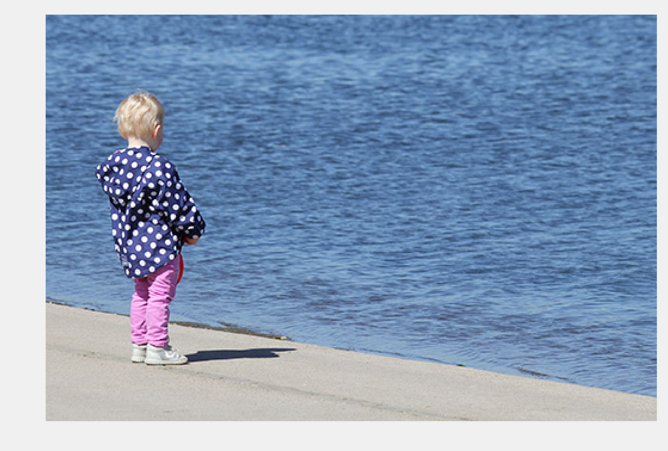
3. We load an image:
img = plt.imread('https://github.com/ipython-books/'
                 'cookbook-2nd-data/blob/master/'
                 'child.png?raw=true')
show(img)
4. Let's find salient points in the image with the Harris corner method. The first step consists of computing the Harris corner measure response image with the corner_harris() function (we will explain this measure in How it works...). This function requires a grayscale image, thus we select the first RGB component:
corners = sf.corner_harris(img[:, :, 0])
show(corners)
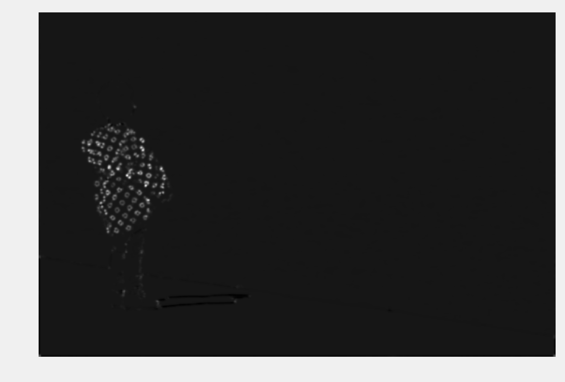
We see that the patterns in the child's coat are well detected by this algorithm.
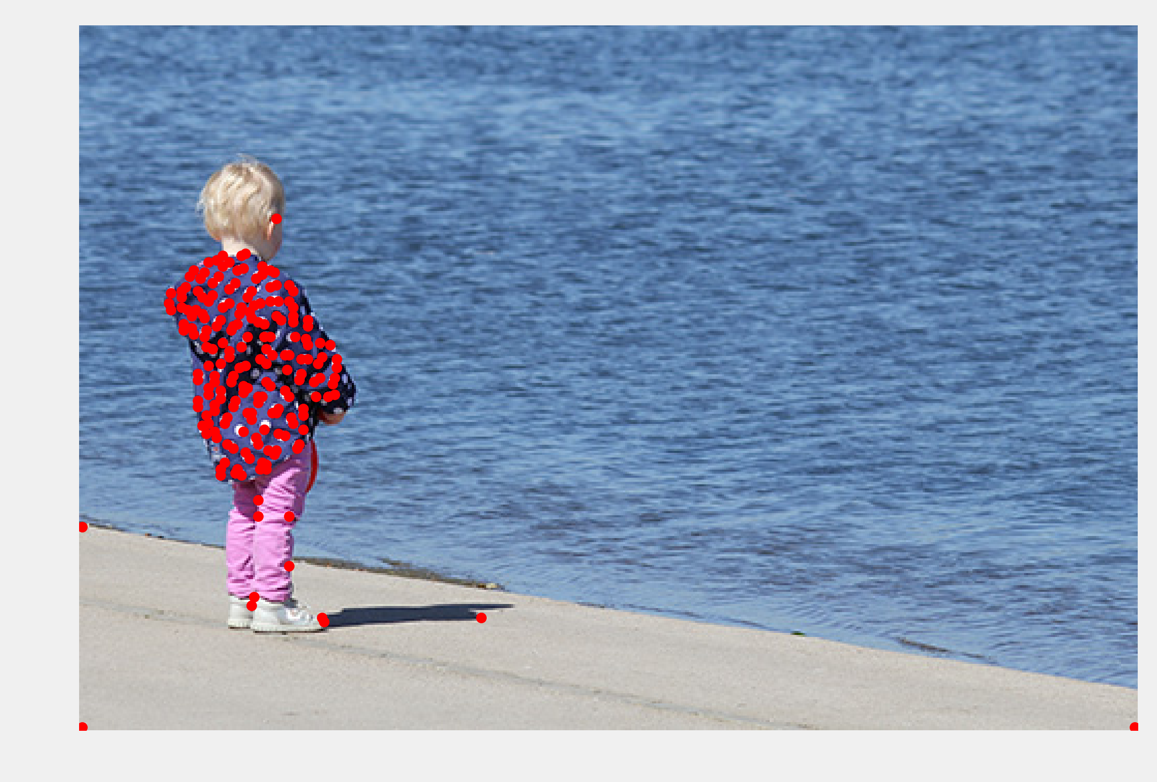
5. The next step is to detect corners from this measure image, using the corner_peaks() function:
peaks = sf.corner_peaks(corners)
ax = show(img)
ax.plot(peaks[:, 1], peaks[:, 0], 'or', ms=4)
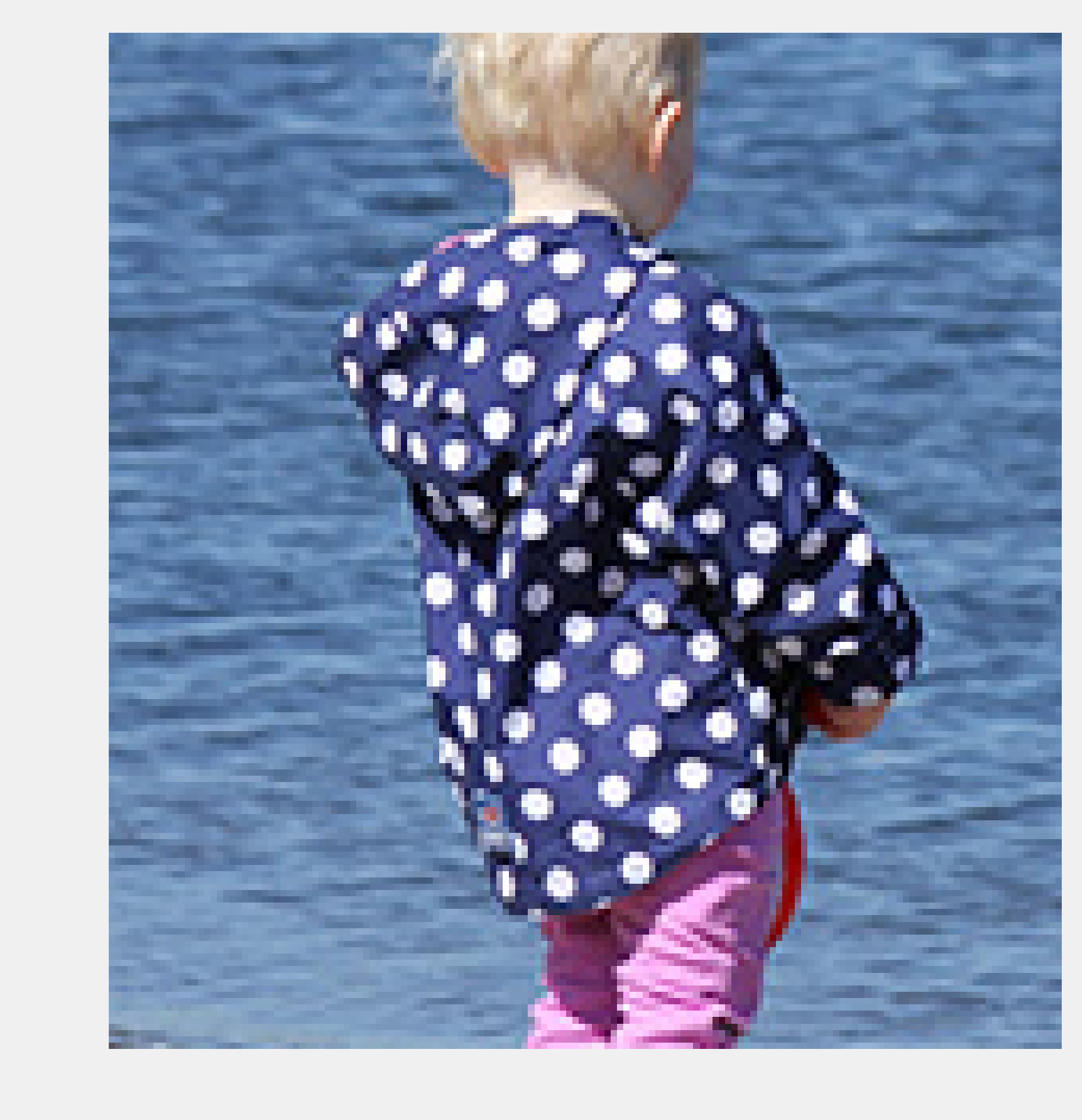
6. Finally, we create a box around the median position of the corner points to define our region of interest:
# The median defines the approximate position of
# the corner points.
ym, xm = np.median(peaks, axis=0)
# The standard deviation gives an estimation
# of the spread of the corner points.
ys, xs = 2 * peaks.std(axis=0)
xm, ym = int(xm), int(ym)
xs, ys = int(xs), int(ys)
show(img[ym - ys:ym + ys, xm - xs:xm + xs])
How it works...
Let's explain the method used in this recipe. The first step consists of computing the structure tensor (or Harris matrix) of the image:
Here, \(I(x, y)\) is the image, \(I_x\) and \(I_y\) are the partial derivatives, and the brackets denote the local spatial average around neighboring values.
This tensor associates a \((2,2)\) positive symmetric matrix at each point. This matrix is used to calculate a sort of autocorrelation of the image at each point.
Let \(\lambda\) and \(\mu\) be the two eigenvalues of this matrix (the matrix is diagonalizable because it is real and symmetric). Roughly, a corner is characterized by a large variation of the autocorrelation in all directions, or in large positive eigenvalues \(\lambda\) and \(\mu\). The corner measure image is defined as:
Here, \(k\) is a tunable parameter. \(M\) is large when there is a corner. Finally, corner_peaks() finds corner points by looking at local maxima in the corner measure image.
There's more...
Here are a few references:
- A corner detection example with scikit-image available at http://scikit-image.org/docs/dev/auto_examples/features_detection/plot_corner.html
- An image processing tutorial with scikit-image available at http://blog.yhathq.com/posts/image-processing-with-scikit-image.html
- Corner detection on Wikipedia, available at https://en.wikipedia.org/wiki/Corner_detection
- Structure tensor on Wikipedia, available at https://en.wikipedia.org/wiki/Structure_tensor
- API reference of the skimage.feature module available at http://scikit-image.org/docs/dev/api/skimage.feature.html