11.2. Applying filters on an image
 This is one of the 100+ free recipes of the IPython Cookbook, Second Edition, by Cyrille Rossant, a guide to numerical computing and data science in the Jupyter Notebook. The ebook and printed book are available for purchase at Packt Publishing.
▶ Text on GitHub with a CC-BY-NC-ND license
▶ Code on GitHub with a MIT license
▶ Go to Chapter 11 : Image and Audio Processing
▶ Get the Jupyter notebook
In this recipe, we apply filters on an image for various purposes: blurring, denoising, and edge detection.
How it works...
1. Let's import the packages:
import numpy as np
import matplotlib.pyplot as plt
import skimage
import skimage.color as skic
import skimage.filters as skif
import skimage.data as skid
import skimage.util as sku
%matplotlib inline
2. We create a function that displays a grayscale image:
def show(img):
    fig, ax = plt.subplots(1, 1, figsize=(8, 8))
    ax.imshow(img, cmap=plt.cm.gray)
    ax.set_axis_off()
    plt.show()
3. Now, we load the Astronaut image (bundled in scikit-image). We convert it to a grayscale image with the rgb2gray() function:
img = skic.rgb2gray(skid.astronaut())
show(img)

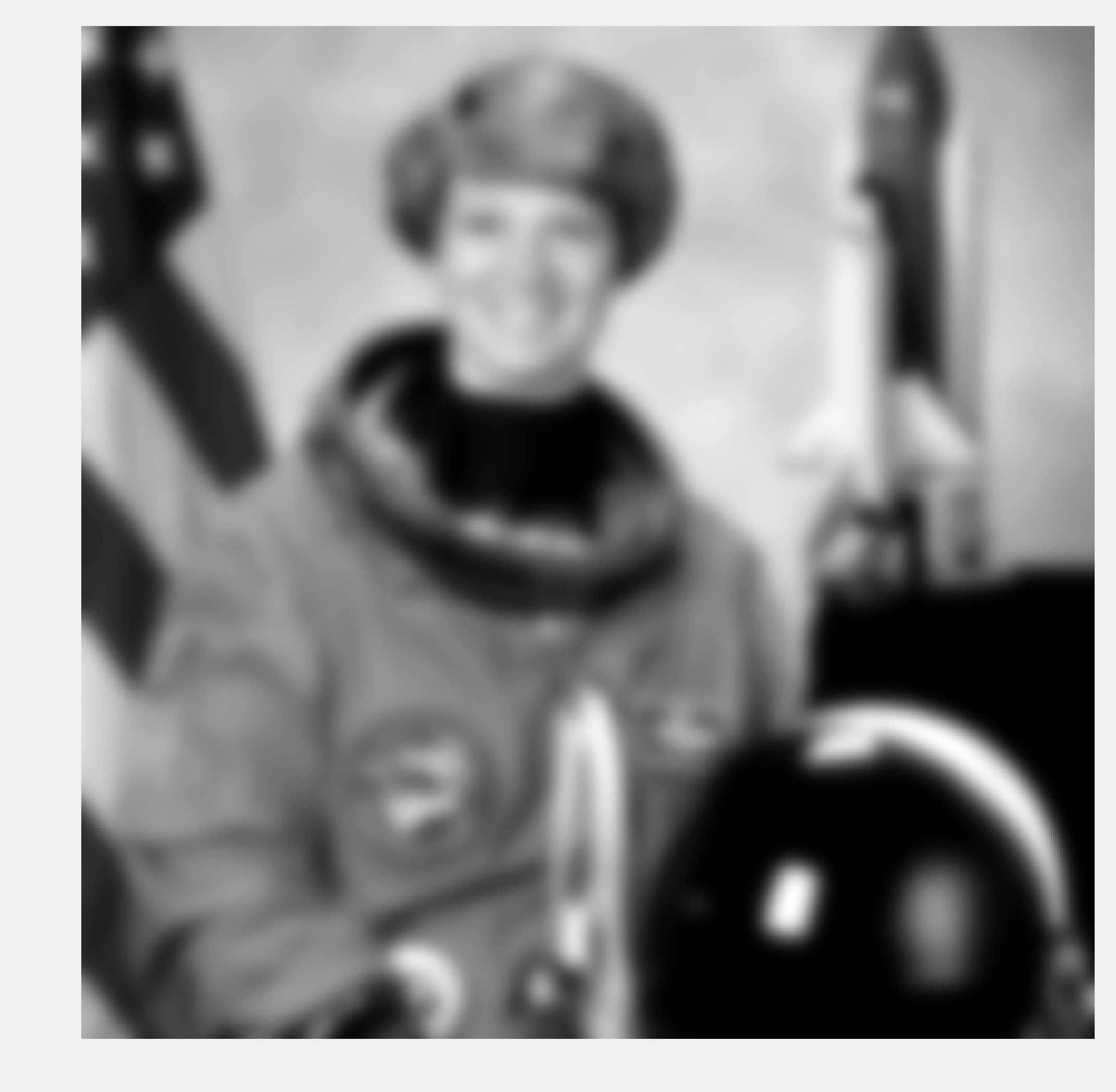
4. Let's apply a blurring Gaussian filter to the image:
show(skif.gaussian(img, 5.))
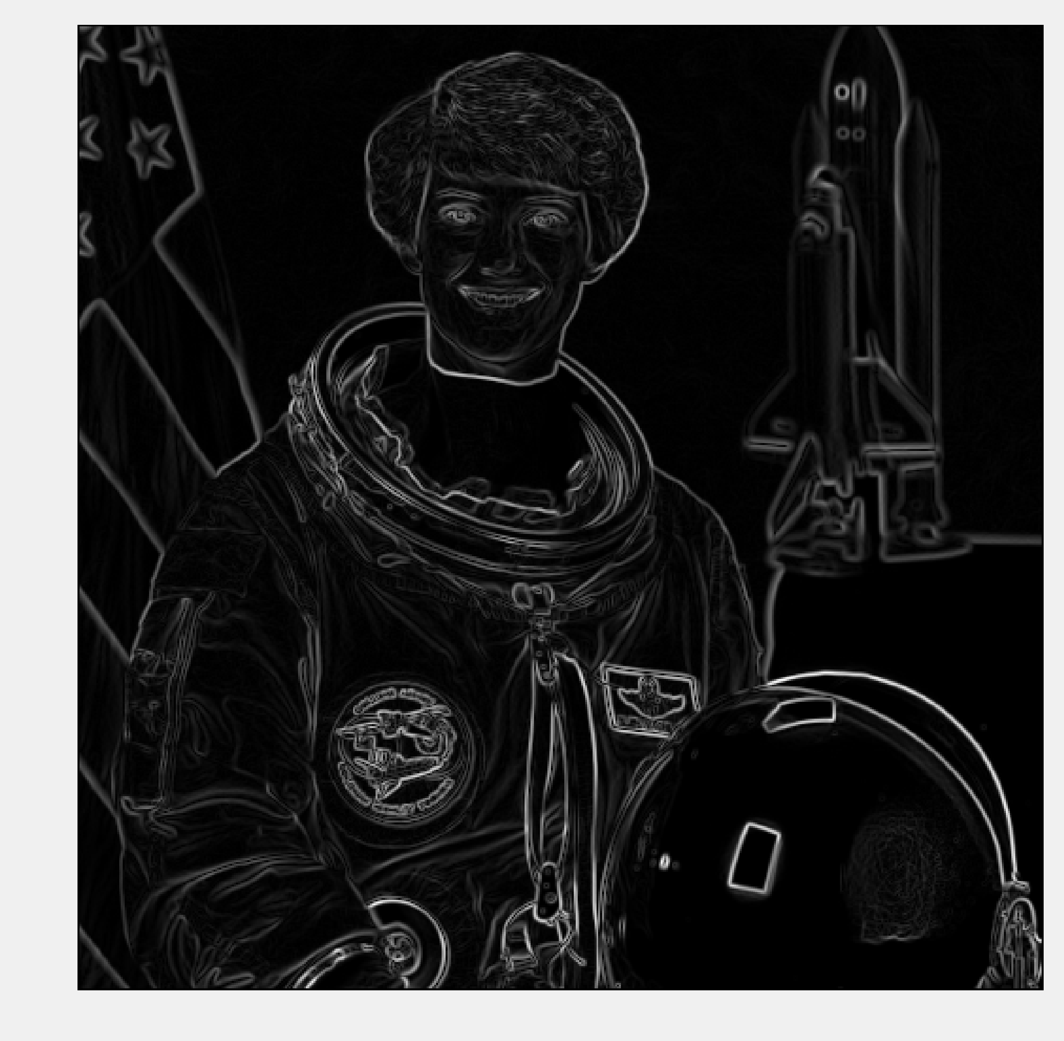
5. We now apply a Sobel filter that enhances the edges in the image:
sobimg = skif.sobel(img)
show(sobimg)
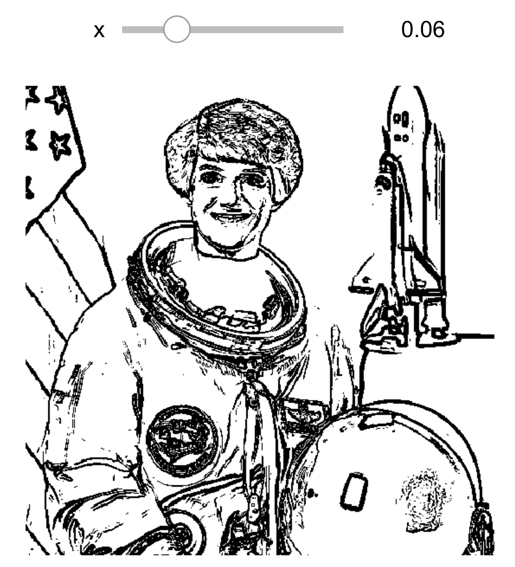
6. We can threshold the filtered image to get a sketch effect. We obtain a binary image that only contains the edges. We use a Notebook widget to find an adequate thresholding value; by adding the @interact decorator, we display a slider on top of the image. This widget lets us control the threshold dynamically.
from ipywidgets import widgets

@widgets.interact(x=(0.01, .2, .005))
def edge(x):
    show(sobimg < x)
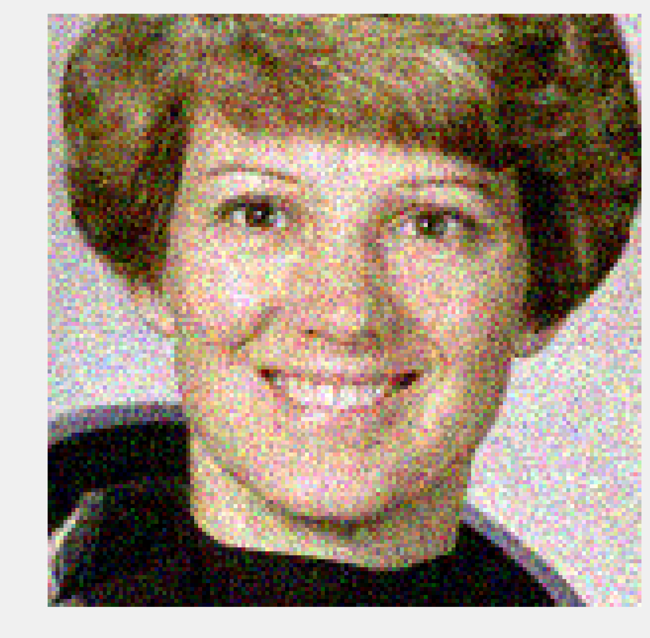
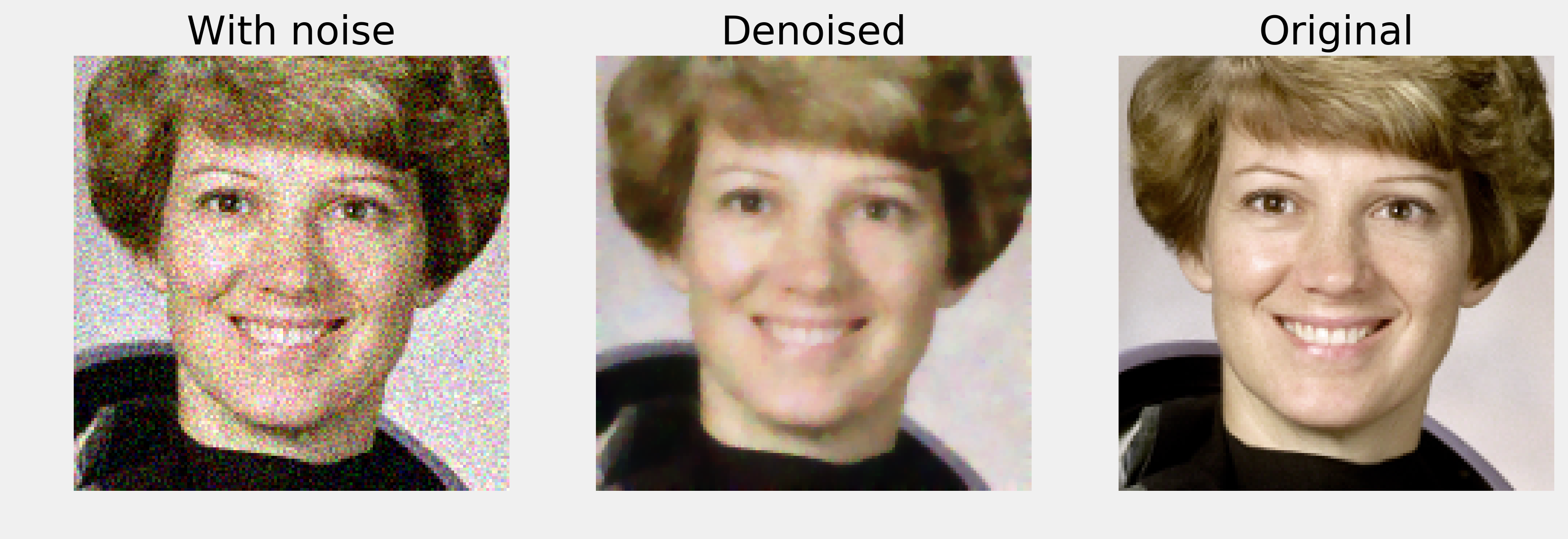
7. Finally, we add some noise to the image to illustrate the effect of a denoising filter:
img = skimage.img_as_float(skid.astronaut())

# We take a portion of the image to show the details.
img = img[50:200, 150:300]

# We add Gaussian noise.
img_n = sku.random_noise(img)
show(img_n)
8. The denoise_tv_bregman() function implements total-variation denoising using the Split Bregman method:
img_r = skimage.restoration.denoise_tv_bregman(
    img_n, 5.)

fig, (ax1, ax2, ax3) = plt.subplots(
    1, 3, figsize=(12, 8))

ax1.imshow(img_n)
ax1.set_title('With noise')
ax1.set_axis_off()

ax2.imshow(img_r)
ax2.set_title('Denoised')
ax2.set_axis_off()

ax3.imshow(img)
ax3.set_title('Original')
ax3.set_axis_off()
How it works...
Many filters used in image processing are linear filters. These filters are very similar to those seen in Chapter 10, Signal Processing; the only difference is that they work in two dimensions. Applying a linear filter to an image amounts to performing a discrete convolution of the image with a particular function. The Gaussian filter applies a convolution with a Gaussian function to blur the image.
The Sobel filter computes an approximation of the gradient of the image. Therefore, it can detect fast-varying spatial changes in the image, which generally correspond to edges.
Image denoising refers to the process of removing noise from an image. Total variation denoising works by finding a regular image close to the original (noisy) image. Regularity is quantified by the total variation of the image:
The Split Bregman method is a variant based on the L1 norm. It is an instance of compressed sensing, which aims to find regular and sparse approximations of real-world noisy measurements.
There's more...
Here are a few references:
- API reference of the skimage.filter module available at http://scikit-image.org/docs/dev/api/skimage.filters.html
- Noise reduction on Wikipedia, available at https://en.wikipedia.org/wiki/Noise_reduction
- Gaussian filter on Wikipedia, available at https://en.wikipedia.org/wiki/Gaussian_filter
- Sobel filter on Wikipedia, available at https://en.wikipedia.org/wiki/Sobel_operator
- The Split Bregman algorithm explained at http://www.ece.rice.edu/~tag7/Tom_Goldstein/Split_Bregman.html
See also
- Manipulating the exposure of an image