IPython Cookbook - 1.1. Introducing IPython and the Jupyter Notebook

This is one of the 100+ free recipes of the IPython Cookbook, Second Edition, by Cyrille Rossant, a guide to numerical computing and data science in the Jupyter Notebook. The ebook and printed book are available for purchase at Packt Publishing.

▶ Text on GitHub with a CC-BY-NC-ND license
▶ Code on GitHub with a MIT license

▶ Go to Chapter 1 : A Tour of Interactive Computing with Jupyter and IPython
▶ Get the Jupyter notebook

The Jupyter Notebook is a web-based interactive environment that combines code, rich text, images, videos, animations, mathematical equations, plots, maps, interactive figures and widgets, and graphical user interfaces, into a single document. This tool is an ideal gateway to high-performance numerical computing and data science in Python, R, Julia, or other languages. In this book, we will mostly use the Python language, although there are recipes introducing R and Julia.

In this recipe, we give an introduction to IPython and the Jupyter Notebook.

Getting ready

This chapter's introduction gives the instructions to install the Anaconda distribution, which comes with Jupyter and almost all Python libraries we will be using in this book.

Once Anaconda is installed, download the code from the book's website and open a terminal in that folder. In the terminal, type jupyter notebook. Your default web browser should open automatically and load the address http://localhost:8888 (a server that runs on your computer). You're ready to get started!

How to do it...

1. Let's create a new Jupyter notebook using an IPython kernel. We type the following command in a cell, and press Shift + Enter to evaluate it:

print("Hello world!")

Hello world!

Screenshot of a Jupyter notebook

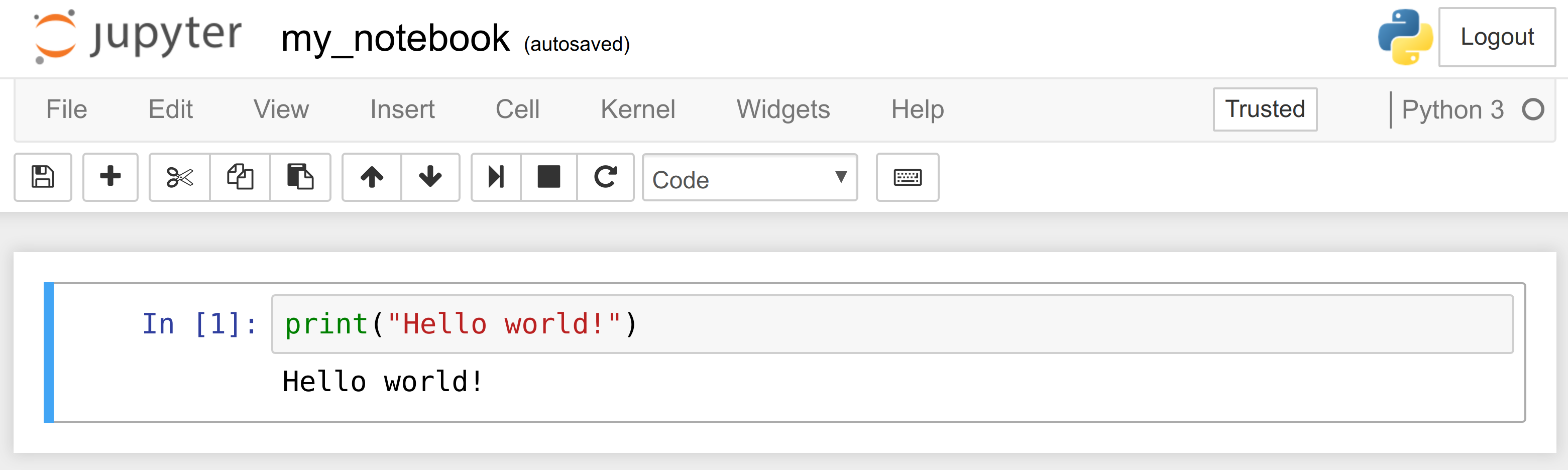
A notebook contains a linear succession of cells and output areas. A cell contains Python code, in one or multiple lines. The output of the code is shown in the corresponding output area.

In this book, the prompt >>> means that you need to type everything that starts after it. The >>> characters themselves should not be typed.

2. Now, we do a simple arithmetic operation:

2 + 2

The result of the operation is shown in the output area. More precisely, the output area not only displays text that is printed by any command in the cell, but it also displays a text representation of the last returned object. Here, the last returned object is the result of 2+2, that is, 4.

3. In the next cell, we can recover the value of the last returned object with the _ (underscore) special variable. In practice, it might be more convenient to assign objects to named variables such as in myresult = 2 + 2.

_ * 3

4. IPython not only accepts Python code, but also shell commands. These commands are provided by the operating system. We first type ! in a cell before typing the shell command. Here, assuming a Linux or macOS system, we get the list of all the notebooks in the current directory:

!ls

my_notebook.ipynb

On Windows, one may replaces ls by dir.

5. IPython comes with a library of magic commands. These commands are convenient shortcuts to common actions. They all start with % (the percent character). We can get the list of all magic commands with %lsmagic:

%lsmagic

Available line magics:
%alias  %alias_magic  %autocall  %automagic  %autosave  %bookmark  %cat  %cd  %clear  %colors  %config  %connect_info  %cp  %debug  %dhist  %dirs  %doctest_mode  %ed  %edit  %env  %gui  %hist  %history  %killbgscripts  %ldir  %less  %lf  %lk  %ll  %load  %load_ext  %loadpy  %logoff  %logon  %logstart  %logstate  %logstop  %ls  %lsmagic  %lx  %macro  %magic  %man  %matplotlib  %mkdir  %more  %mv  %notebook  %page  %pastebin  %pdb  %pdef  %pdoc  %pfile  %pinfo  %pinfo2  %popd  %pprint  %precision  %profile  %prun  %psearch  %psource  %pushd  %pwd  %pycat  %pylab  %qtconsole  %quickref  %recall  %rehashx  %reload_ext  %rep  %rerun  %reset  %reset_selective  %rm  %rmdir  %run  %save  %sc  %set_env  %store  %sx  %system  %tb  %time  %timeit  %unalias  %unload_ext  %who  %who_ls  %whos  %xdel  %xmode

Available cell magics:
%%!  %%HTML  %%SVG  %%bash  %%capture  %%debug  %%file  %%html  %%javascript  %%js  %%latex  %%markdown  %%perl  %%prun  %%pypy  %%python  %%python2  %%python3  %%ruby  %%script  %%sh  %%svg  %%sx  %%system  %%time  %%timeit  %%writefile

Automagic is ON, % prefix IS NOT needed for line magics.

Cell magics have a %% prefix; they target entire code cells.

6. For example, the %%writefile cell magic lets us create a text file. This magic command accepts a filename as an argument. All the remaining lines in the cell are directly written to this text file. Here, we create a file test.txt and write Hello world! into it:

%%writefile test.txt
Hello world!

Writing test.txt

# Let's check what this file contains.
with open('test.txt', 'r') as f:
    print(f.read())

Hello world!

7. As we can see in the output of %lsmagic, there are many magic commands in IPython. We can find more information about any command by adding ? after it. For example, to get some help about the %run magic command, we type %run?as shown here:

%run?

Screenshot of the pager

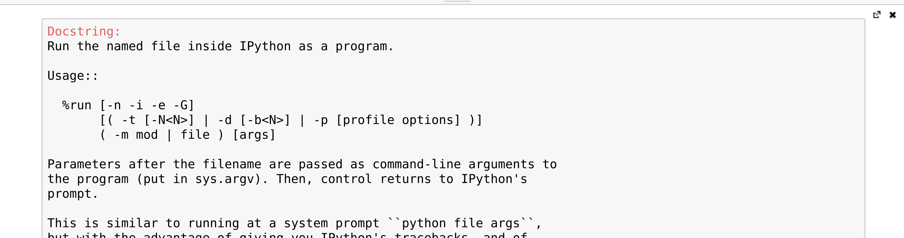
The pager (a text area at the bottom of the screen) opens and shows the help of the %run magic command.

8. We covered the basics of IPython and the Notebook. Let's now turn to the rich display and interactive features of the Notebook. Until now, we have only created code cells (containing code). Jupyter supports other types of cells. In the Notebook toolbar, there is a drop-down menu to select the cell's type. The most common cell type after the code cell is the Markdown cell.

Markdown cells contain rich text formatted with Markdown, a popular plain text- formatting syntax. This format supports normal text, headers, bold, italics, hypertext links, images, mathematical equations in LaTeX (a typesetting system adapted to mathematics), code, HTML elements, and other features, as shown here:

Markdown cell

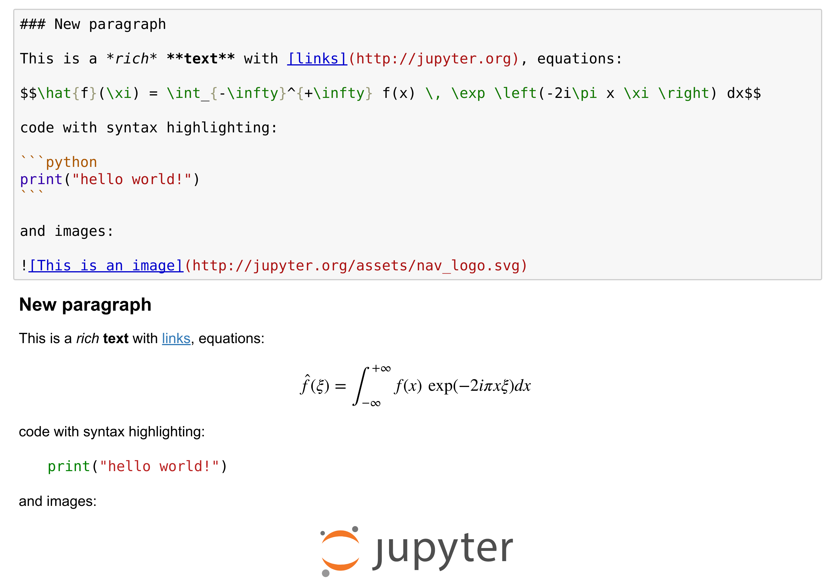
Running a Markdown cell (by pressing Shift + Enter, for example) displays the output, as shown in the bottom panel of the screenshot above.

By combining code cells and Markdown cells, we create a standalone interactive document that combines computations (code), text and graphics.

9. The Jupyter Notebook also comes with a sophisticated display system that lets us insert rich web elements in the Notebook. Here, we show how to add HTML, SVG (Scalable Vector Graphics), and even YouTube videos in a notebook. First, we need to import some classes:

from IPython.display import HTML, SVG, YouTubeVideo

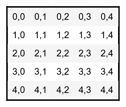
10. We create an HTML table dynamically with Python, and we display it in the (HTML-based) notebook.

HTML('''
<table style="border: 2px solid black;">
''' +
     ''.join(['<tr>' +
              ''.join([f'<td>{row},{col}</td>'
                       for col in range(5)]) +
              '</tr>' for row in range(5)]) +
     '''
</table>
''')

<IPython.core.display.HTML object>

11. Similarly, we create an SVG graphics dynamically:

SVG('''<svg width="600" height="80">''' +
    ''.join([f'''<circle
              cx="{(30 + 3*i) * (10 - i)}"
              cy="30"
              r="{3. * float(i)}"
              fill="red"
              stroke-width="2"
              stroke="black">
        </circle>''' for i in range(10)]) +
    '''</svg>''')

<IPython.core.display.SVG object>

12. We display a Youtube video by giving its identifier to YoutubeVideo:

YouTubeVideo('VQBZ2MqWBZI')

<IPython.lib.display.YouTubeVideo at 0x7fc0000b64a8>

There's more...

Notebooks are saved as structured text files (JSON format), which makes them easily shareable. Here are the contents of a simple notebook:

{
 "cells": [
  {
   "cell_type": "code",
   "execution_count": 1,
   "metadata": {},
   "outputs": [
    {
     "name": "stdout",
     "output_type": "stream",
     "text": [
      "Hello world!\n"
     ]
    }
   ],
   "source": [
    "print(\"Hello world!\")"
   ]
  }
 ],
 "metadata": {},
 "nbformat": 4,
 "nbformat_minor": 2
}

Jupyter comes with a special tool, nbconvert, which converts notebooks to other formats such as HTML and PDF (https://nbconvert.readthedocs.io/en/stable/).

Another online tool, nbviewer (http://nbviewer.jupyter.org), allows us to render a publicly-available notebook directly in the browser.

We will cover many of these possibilities in the subsequent chapters, notably in Chapter 3, Mastering the Notebook.

There are other implementations of Jupyter Notebook frontends that offer different ways of interacting with the same notebook documents. Jupyterlab, an IDE for interactive computing and data science, is the future of the Jupyter Notebook. It is introduced in Chapter 3. nteract is a desktop application that lets the user open a notebook file by double-clicking on it, without using the terminal and using a web browser. Hydrogen is a plugin of the Atom text editor that provides rich interactive capabilities when opening notebook files. Juno is a Jupyter Notebook client for iPad.

Here are a few references about the Notebook:

Installing Jupyter, available at http://jupyter.org/install.html
Documentation of the Notebook available at http://jupyter.readthedocs.io/en/latest/index.html
Security in Jupyter notebooks, at https://jupyter-notebook.readthedocs.io/en/stable/security.html#Security-in-notebook-documents
User-curated gallery of interesting notebooks available at https://github.com/jupyter/jupyter/wiki/A-gallery-of-interesting-Jupyter-Notebooks
JupyterLab at https://github.com/jupyterlab/jupyterlab
nteract at https://nteract.io
Hydrogen at https://nteract.io/atom
Juno at https://juno.sh/

Getting ready

How to do it...

There's more...

See also