7.6. Estimating a probability distribution nonparametrically with a kernel density estimation
 This is one of the 100+ free recipes of the IPython Cookbook, Second Edition, by Cyrille Rossant, a guide to numerical computing and data science in the Jupyter Notebook. The ebook and printed book are available for purchase at Packt Publishing.
▶ Text on GitHub with a CC-BY-NC-ND license
▶ Code on GitHub with a MIT license
▶ Go to Chapter 7 : Statistical Data Analysis
▶ Get the Jupyter notebook
In the previous recipe, we applied a parametric estimation method. We had a statistical model (the exponential distribution) describing our data, and we estimated a single parameter (the rate of the distribution). Nonparametric estimation deals with statistical models that do not belong to a known family of distributions. The parameter space is then infinite-dimensional instead of finite-dimensional (that is, we estimate functions rather than numbers).
Here, we use a kernel density estimation (KDE) to estimate the density of probability of a spatial distribution. We look at the geographical locations of tropical cyclones from 1848 to 2013, based on data provided by the NOAA, the US' National Oceanic and Atmospheric Administration.
Getting ready
You need cartopy, available at http://scitools.org.uk/cartopy/. You can install it with conda install -c conda-forge cartopy.
How to do it...
1. Let's import the usual packages. The kernel density estimation with a Gaussian kernel is implemented in scipy.stats:
import numpy as np
import pandas as pd
import scipy.stats as st
import matplotlib.pyplot as plt
from matplotlib.colors import ListedColormap
import cartopy.crs as ccrs
%matplotlib inline
2. Let's open the data with pandas:
# www.ncdc.noaa.gov/ibtracs/index.php?name=wmo-data
df = pd.read_csv('https://github.com/ipython-books/'
                 'cookbook-2nd-data/blob/master/'
                 'Allstorms.ibtracs_wmo.v03r05.csv?'
                 'raw=true')
3. The dataset contains information about most storms since 1848. A single storm may appear multiple times across several consecutive days.
df[df.columns[[0, 1, 3, 8, 9]]].head()
4. We use pandas' groupby() function to obtain the average location of every storm:
dfs = df.groupby('Serial_Num')
pos = dfs[['Latitude', 'Longitude']].mean()
x = pos.Longitude.values
y = pos.Latitude.values
pos.head()
5. We display the storms on a map with cartopy. This toolkit allows us to easily project the geographical coordinates on the map.
# We use a simple equirectangular projection,
# also called Plate Carree.
geo = ccrs.Geodetic()
crs = ccrs.PlateCarree()
# We create the map plot.
ax = plt.axes(projection=crs)
# We display the world map picture.
ax.stock_img()
# We display the storm locations.
ax.scatter(x, y, color='r', s=.5, alpha=.25, transform=geo)
6. Before performing the kernel density estimation, we transform the storms' positions from the geodetic coordinate system (longitude and latitude) into the map's coordinate system, called plate carrée.
h = crs.transform_points(geo, x, y)[:, :2].T
h.shape
(2, 6940)
7. Now, we perform the kernel density estimation on our (2, N) array.
kde = st.gaussian_kde(h)
8. The gaussian_kde() routine returned a Python function. To see the results on a map, we need to evaluate this function on a 2D grid spanning the entire map. We create this grid with meshgrid(), and we pass the x and y values to the kde() function:
k = 100
# Coordinates of the four corners of the map.
x0, x1, y0, y1 = ax.get_extent()
# We create the grid.
tx, ty = np.meshgrid(np.linspace(x0, x1, 2 * k),
                     np.linspace(y0, y1, k))
# We reshape the grid for the kde() function.
mesh = np.vstack((tx.ravel(), ty.ravel()))
# We evaluate the kde() function on the grid.
v = kde(mesh).reshape((k, 2 * k))
9. Before displaying the KDE heatmap on the map, we need to use a special colormap with a transparent channel. This will allow us to superimpose the heatmap on the stock image:
# [https://stackoverflow.com/a/37334212/1595060](https://stackoverflow.com/a/37334212/1595060)
cmap = plt.get_cmap('Reds')
my_cmap = cmap(np.arange(cmap.N))
my_cmap[:, -1] = np.linspace(0, 1, cmap.N)
my_cmap = ListedColormap(my_cmap)
10. Finally, we display the estimated density with imshow():
ax = plt.axes(projection=crs)
ax.stock_img()
ax.imshow(v, origin='lower',
          extent=[x0, x1, y0, y1],
          interpolation='bilinear',
          cmap=my_cmap)
How it works...
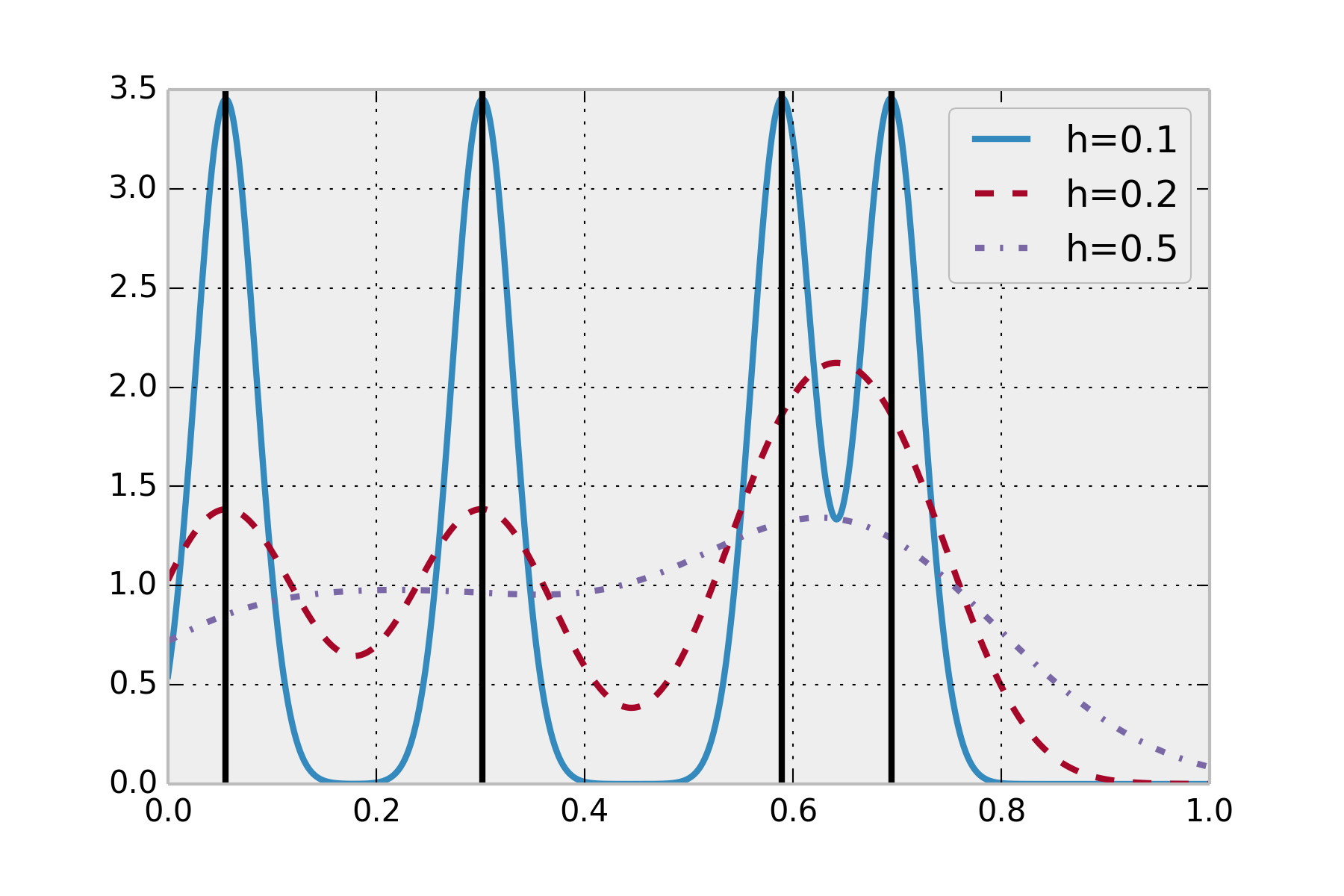
The kernel density estimator of a set of n points \(\{x_i\}\) is given as:
Here, \(h>0\) is a scaling parameter (the bandwidth) and \(K(u)\) is the kernel, a symmetric function that integrates to 1. This estimator is to be compared with a classical histogram, where the kernel would be a top-hat function (a rectangle function taking its values in \(\{0,1\}\)), but the blocks would be located on a regular grid instead of the data points. For more information on kernel density estimator, refer to https://en.wikipedia.org/wiki/Kernel_density_estimation.
Multiple kernels can be chosen. Here, we chose a Gaussian kernel, so that the KDE is the superposition of Gaussian functions centered on all the data points. It is an estimation of the density.
The choice of the bandwidth is not trivial; there is a tradeoff between a too low value (small bias, high variance: overfitting) and a too high value (high bias, small variance: underfitting). We will return to this important concept of bias-variance tradeoff in the next chapter. For more information on the bias-variance tradeoff, refer to https://en.wikipedia.org/wiki/Bias-variance_dilemma.
There are several methods to automatically choose a sensible bandwidth. SciPy uses a rule of thumb called Scott's Rule: h = n**(-1. / (d + 4)). You will find more information at http://scipy.github.io/devdocs/generated/scipy.stats.gaussian_kde.html.
The following figure illustrates the KDE. The sample dataset contains four points in \([0,1]\) (black lines). The estimated density is a smooth curve, represented here with different bandwidth values.
There are other implementations of KDE in statsmodels and scikit-learn. You can find more information here: http://jakevdp.github.io/blog/2013/12/01/kernel-density-estimation/
See also
- Fitting a probability distribution to data with the maximum likelihood method