6.3. Creating interactive Web visualizations with Bokeh and HoloViews
 This is one of the 100+ free recipes of the IPython Cookbook, Second Edition, by Cyrille Rossant, a guide to numerical computing and data science in the Jupyter Notebook. The ebook and printed book are available for purchase at Packt Publishing.
▶ Text on GitHub with a CC-BY-NC-ND license
▶ Code on GitHub with a MIT license
▶ Go to Chapter 6 : Data Visualization
▶ Get the Jupyter notebook
Bokeh (http://bokeh.pydata.org/en/latest/) is a library for creating rich interactive visualizations in a browser. Plots are designed in Python, and they are rendered in the browser.
In this recipe, we will give a few examples of interactive Bokeh figures in the Jupyter Notebook. We will also introduce HoloViews which provides a high-level API for bokeh and other plotting libraries.
Getting ready
Bokeh should be installed by default in Anaconda, but you can also install it manually by typing conda install bokeh in a terminal.
To install HoloViews, type conda install -c ioam holoviews.
How to do it...
1. Let's import NumPy and Bokeh. We need to call output_notebook() to tell Bokeh to render plots in the Jupyter Notebook.
import numpy as np
import pandas as pd
import bokeh
import bokeh.plotting as bkh
bkh.output_notebook()
2. Let's create a scatter plot of random data:
f = bkh.figure(width=600, height=400)
f.circle(np.random.randn(1000),
         np.random.randn(1000),
         size=np.random.uniform(2, 10, 1000),
         alpha=.5)
bkh.show(f)
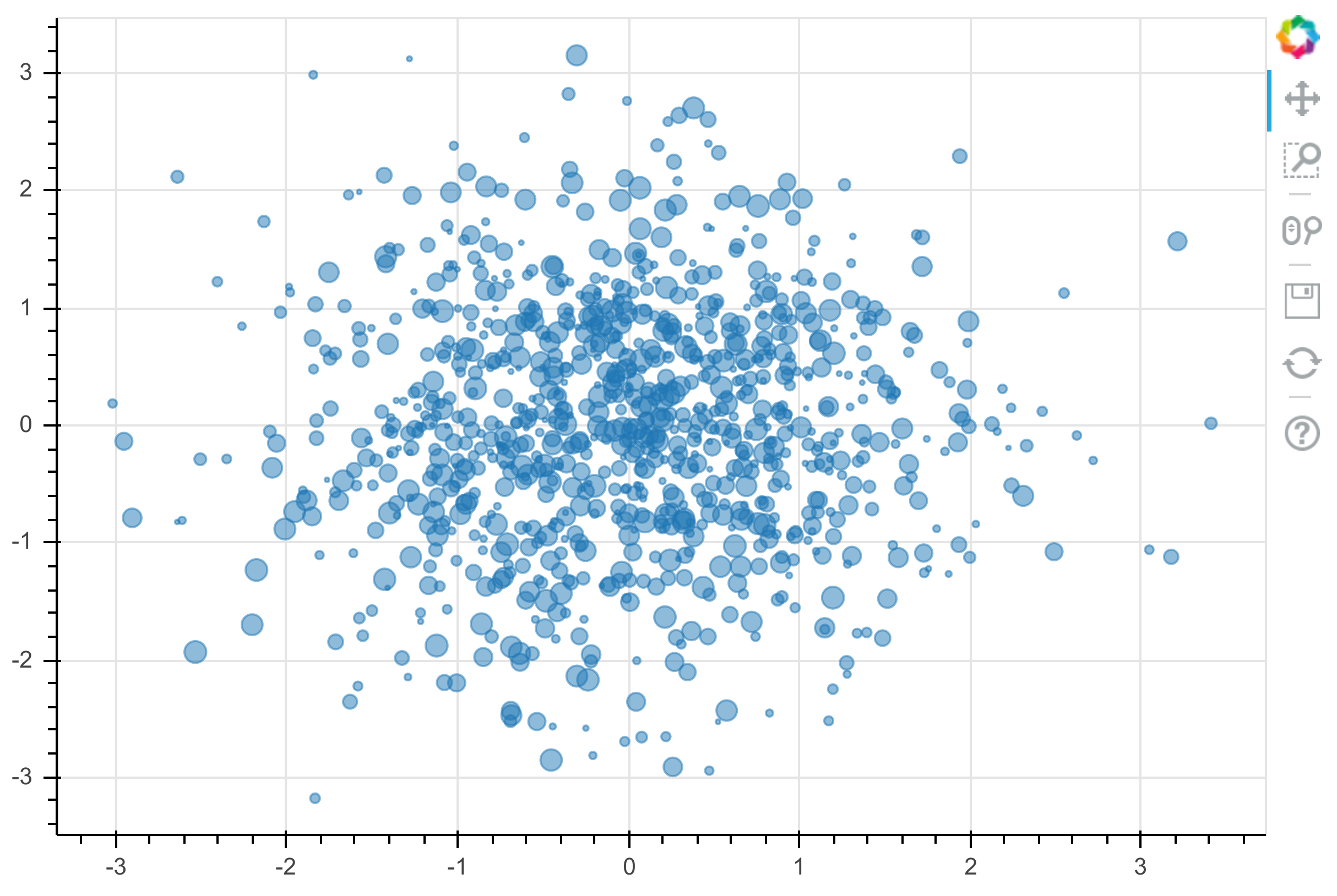
An interactive plot is rendered in the notebook. We can pan and zoom by clicking on the toolbar buttons on the right.
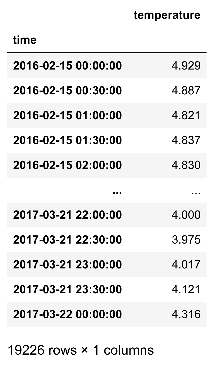
3. Let's load a sample dataset, sea_surface_temperature:
from bokeh.sampledata import sea_surface_temperature
data = sea_surface_temperature.sea_surface_temperature
data
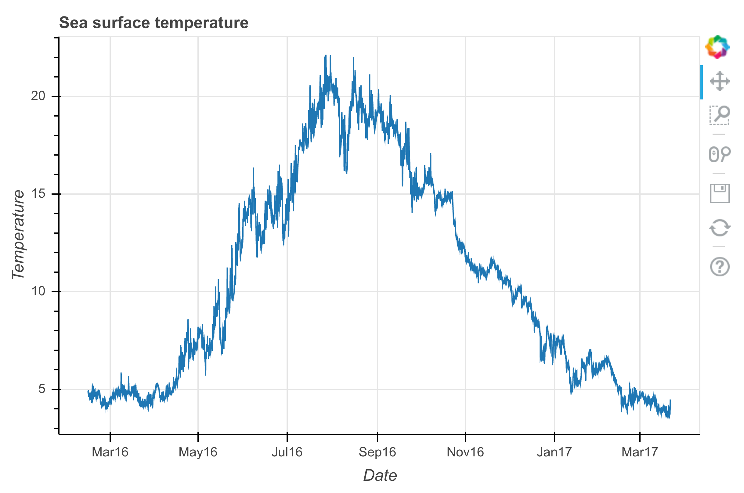
4. Now, we plot the evolution of the temperature as a function of time:
f = bkh.figure(x_axis_type="datetime",
               title="Sea surface temperature",
               width=600, height=400)
f.line(data.index, data.temperature)
f.xaxis.axis_label = "Date"
f.yaxis.axis_label = "Temperature"
bkh.show(f)
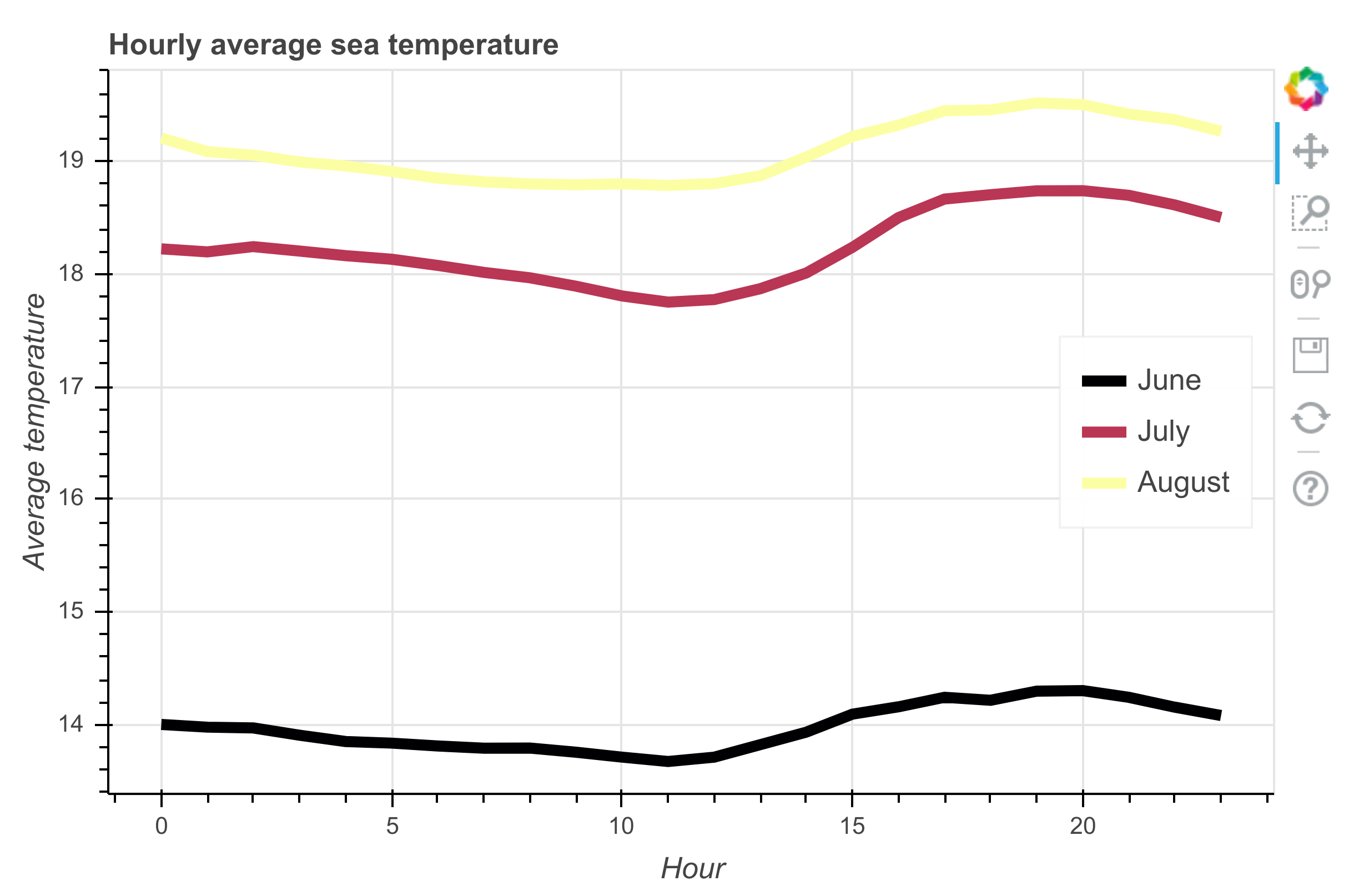
5. We use pandas to plot the hourly average temperature:
months = (6, 7, 8)
data_list = [data[data.index.month == m]
             for m in months]
# We group by the hour of the measure:
data_avg = [d.groupby(d.index.hour).mean()
            for d in data_list]
f = bkh.figure(width=600, height=400,
               title="Hourly average sea temperature")
for d, c, m in zip(data_avg,
                   bokeh.palettes.Inferno[3],
                   ('June', 'July', 'August')):
    f.line(d.index, d.temperature,
           line_width=5,
           line_color=c,
           legend=m,
           )
f.xaxis.axis_label = "Hour"
f.yaxis.axis_label = "Average temperature"
f.legend.location = 'center_right'
bkh.show(f)
6. Let's move to HoloViews:
import holoviews as hv
hv.extension('bokeh')
7. We create a 3D array which could represent a time-dependent 2D image:
data = np.random.rand(100, 100, 10)
ds = hv.Dataset((np.arange(10),
                 np.linspace(0., 1., 100),
                 np.linspace(0., 1., 100),
                 data),
                kdims=['time', 'y', 'x'],
                vdims=['z'])
ds
:Dataset [time,y,x] (z)
The ds object is a Dataset instance representing our time-dependent data. The kdims are the key dimensions (time and space) whereas the vdims are the quantities of interest (here, a scalar z). In other words, the kdims represent the axes of the 3D array data, whereas the vdims represent the values stored in the array.
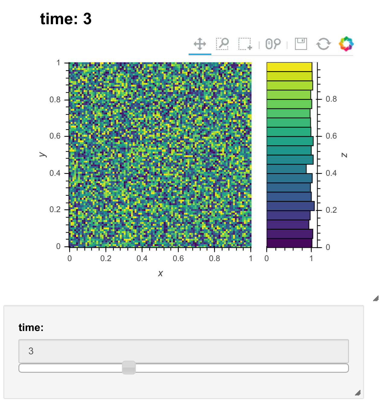
8. We can easily display the 2D image with a slider to change the time, and a histogram of z as a function of time:
%opts Image(cmap='viridis')
ds.to(hv.Image, ['x', 'y']).hist()
There's more...
Bokeh figures in the Notebook are interactive even in the absence of a Python server. For example, our figures can be interactive in nbviewer. Bokeh can also generate standalone HTML/JavaScript documents from our plots. More examples can be found in the gallery.
The xarray library (see http://xarray.pydata.org/en/stable/) provides a way to represent multidimensional arrays with axes. HoloViews can work with xarray objects.
plotly is a company specialized in interactive visualization. They provide an open-source Python visualization library (see https://plot.ly/python/). They also propose tools for building dashboard-style Web-based interfaces (see https://plot.ly/products/dash/).
Datashader (http://datashader.readthedocs.io/en/latest/) and vaex (http://vaex.astro.rug.nl/) are two visualization libraries that target very large datasets.
Here are a few references:
- Bokeh user guide at http://bokeh.pydata.org/en/latest/docs/user_guide.html
- Bokeh gallery at http://bokeh.pydata.org/en/latest/docs/gallery.html
- Using Bokeh in the Notebook, available at http://bokeh.pydata.org/en/latest/docs/user_guide/notebook.html
- HoloViews at http://holoviews.org
- HoloViews gallery at http://holoviews.org/gallery/index.html
- HoloViews tutorial at https://github.com/ioam/jupytercon2017-holoviews-tutorial