4.3. Profiling your code line-by-line with line_profiler

This is one of the 100+ free recipes of the IPython Cookbook, Second Edition, by Cyrille Rossant, a guide to numerical computing and data science in the Jupyter Notebook. The ebook and printed book are available for purchase at Packt Publishing.

▶  Text on GitHub with a CC-BY-NC-ND license
▶  Code on GitHub with a MIT license

▶  Go to Chapter 4 : Profiling and Optimization
▶  Get the Jupyter notebook

Python's native cProfile module and the corresponding %prun magic break down the execution time of code function by function. Sometimes, we may need an even more fine-grained analysis of code performance with a line-by-line report. Such reports can be easier to read than the reports of cProfile.

To profile code line-by-line, we need an external Python module named line_profiler. In this recipe, we will demonstrate how to use this module within IPython.

Getting ready

To install line_profiler, type conda install line_profiler in a terminal.

How do to it...

We will profile the same simulation code as in the previous recipe, line-by-line.

1.  First, let's import NumPy and the line_profiler IPython extension module that comes with the package:

import numpy as np
%load_ext line_profiler

2.  This IPython extension module provides an %lprun magic command to profile a Python function line-by-line. It works best when the function is defined in a file and not in the interactive namespace or in the Notebook. Therefore, here we write our code in a Python script using the %%writefile cell magic:

%%writefile simulation.py
import numpy as np

def step(*shape):
    # Create a random n-vector with +1 or -1 values.
    return 2 * (np.random.random_sample(shape)<.5) - 1

def simulate(iterations, n=10000):
    s = step(iterations, n)
    x = np.cumsum(s, axis=0)
    bins = np.arange(-30, 30, 1)
    y = np.vstack([np.histogram(x[i,:], bins)[0]
                   for i in range(iterations)])
    return y

3.  Now, let's import this script into the interactive namespace so that we can execute and profile our code:

from simulation import simulate

4.  We execute the function under the control of the line profiler. The functions to be profiled need to be explicitly specified in the %lprun magic command. We also save the report in a file named lprof0:

%lprun -T lprof0 -f simulate simulate(50)

*** Profile printout saved to text file 'lprof0'.

5.  Let's display the report:

print(open('lprof0', 'r').read())

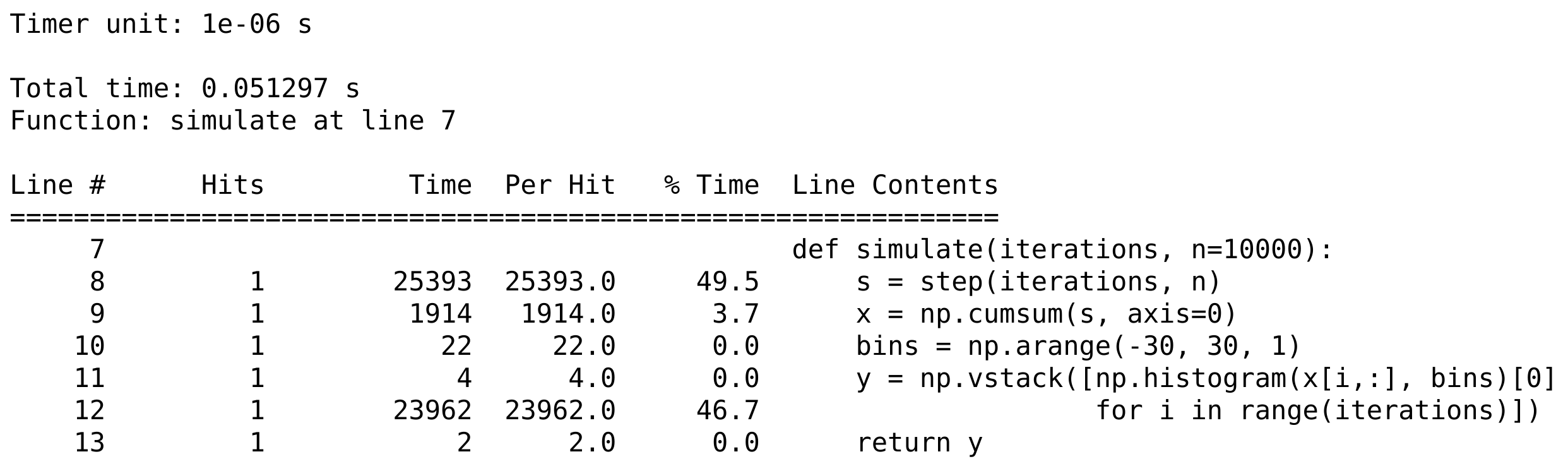
How it works...

The %lprun command accepts a Python statement as its main argument. The functions to profile need to be explicitly specified with -f. Other optional arguments include -D, -T, and -r, and they work in a similar way to their %prun magic command counterparts.

The line_profiler module displays the time spent on each line of the profiled functions, either in timer units or as a fraction of the total execution time. These details are essential when we are looking for hotspots in our code.

There's more...

Tracing is a related method. Python's trace module allows us to trace program execution of Python code. That's particularly useful during in-depth debugging and profiling sessions. We can follow the entire sequence of instructions executed by the Python interpreter. More information on the trace module is available at https://docs.python.org/3/library/trace.html.

In addition, the Online Python Tutor is an online interactive educational tool that can help us understand what the Python interpreter is doing step-by-step as it executes a program's source code. The Online Python Tutor is available at http://pythontutor.com/.

Here are a few references:

• line_profiler repository at https://github.com/rkern/line_profiler

See also

• Profiling your code easily with cProfile and IPython
• Profiling the memory usage of your code with memory_profiler