11.3. Segmenting an image
 This is one of the 100+ free recipes of the IPython Cookbook, Second Edition, by Cyrille Rossant, a guide to numerical computing and data science in the Jupyter Notebook. The ebook and printed book are available for purchase at Packt Publishing.
▶ Text on GitHub with a CC-BY-NC-ND license
▶ Code on GitHub with a MIT license
▶ Go to Chapter 11 : Image and Audio Processing
▶ Get the Jupyter notebook
Image segmentation consists of partitioning an image into different regions that share certain characteristics. This is a fundamental task in computer vision, facial recognition, and medical imaging. For example, an image segmentation algorithm can automatically detect the contours of an organ in a medical image.
scikit-image provides several segmentation methods. In this recipe, we will demonstrate how to segment an image containing different objects. This recipe is inspired by a scikit-image example available at http://scikit-image.org/docs/dev/user_guide/tutorial_segmentation.html
How to do it...
1. Let's import the packages:
import numpy as np
import matplotlib.pyplot as plt
from skimage.data import coins
from skimage.filters import threshold_otsu
from skimage.segmentation import clear_border
from skimage.morphology import label, closing, square
from skimage.measure import regionprops
from skimage.color import lab2rgb
%matplotlib inline
2. We create a function that displays a grayscale image:
def show(img, cmap=None):
    cmap = cmap or plt.cm.gray
    fig, ax = plt.subplots(1, 1, figsize=(8, 6))
    ax.imshow(img, cmap=cmap)
    ax.set_axis_off()
    plt.show()
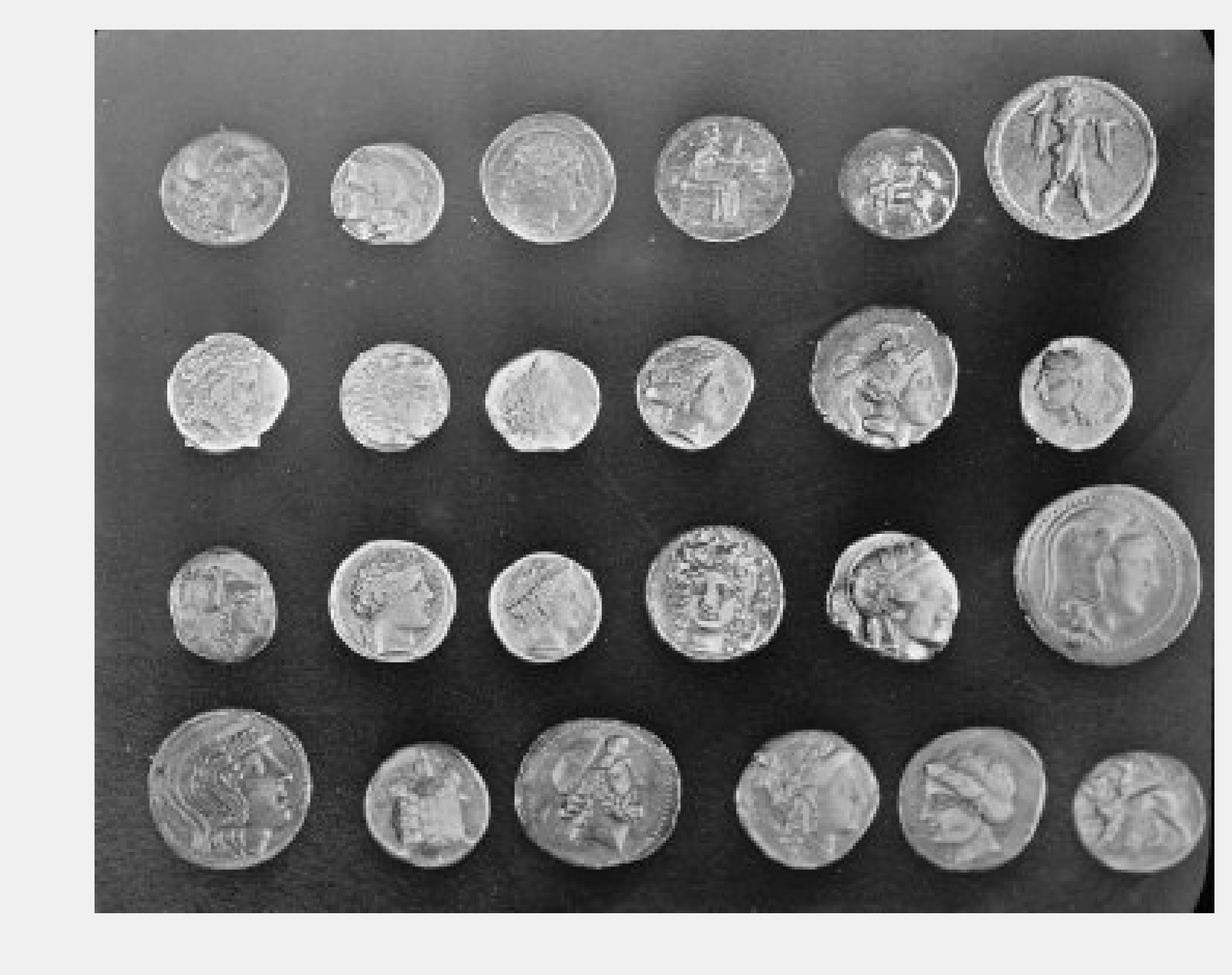
3. We get a test image bundled in scikit-image, showing various coins on a plain background:
img = coins()
show(img)
4. The first step to segment the image is finding an intensity threshold separating the (bright) coins from the (dark) background. Otsu's method defines a simple algorithm to automatically find such a threshold.
threshold_otsu(img)
107
show(img > 107)
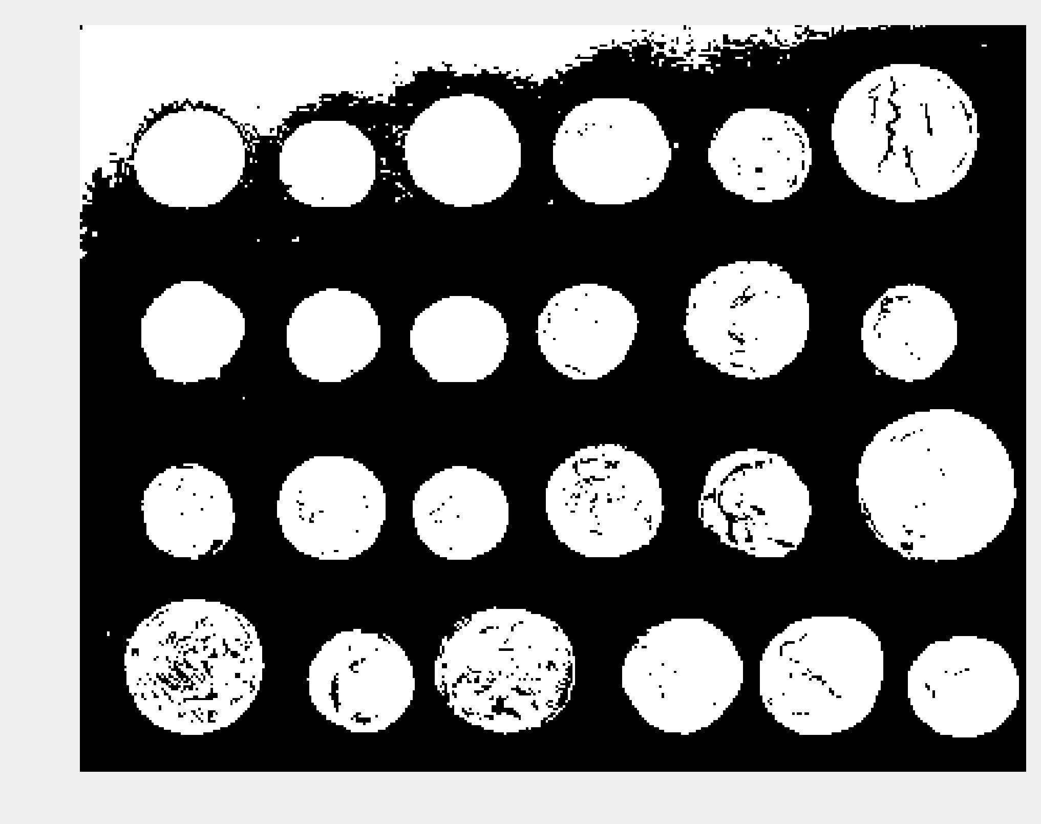
5. There appears to be a problem in the top-left corner of the image, with part of the background being too bright. Let's use a Notebook widget to find a better threshold:
from ipywidgets import widgets

@widgets.interact(t=(50, 240))
def threshold(t):
    show(img > t)
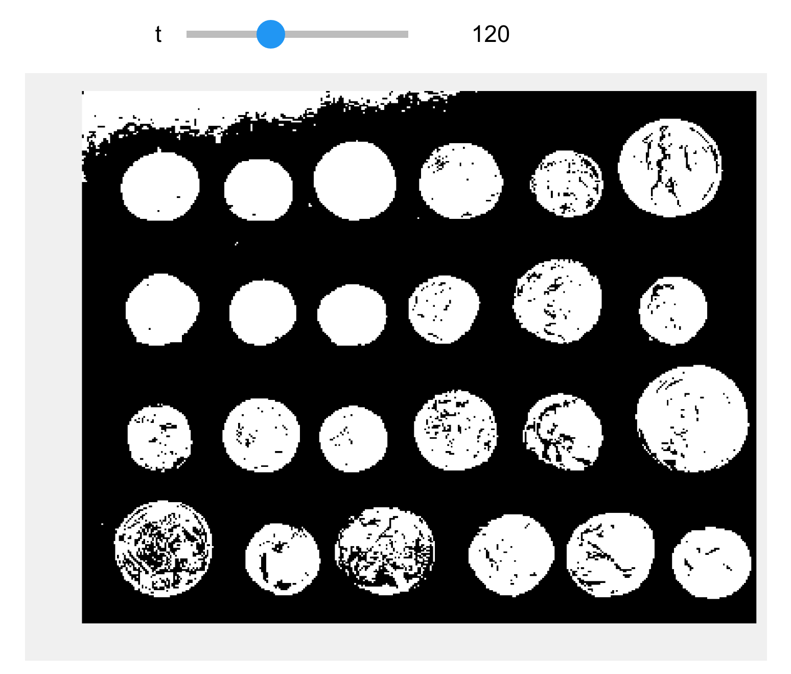
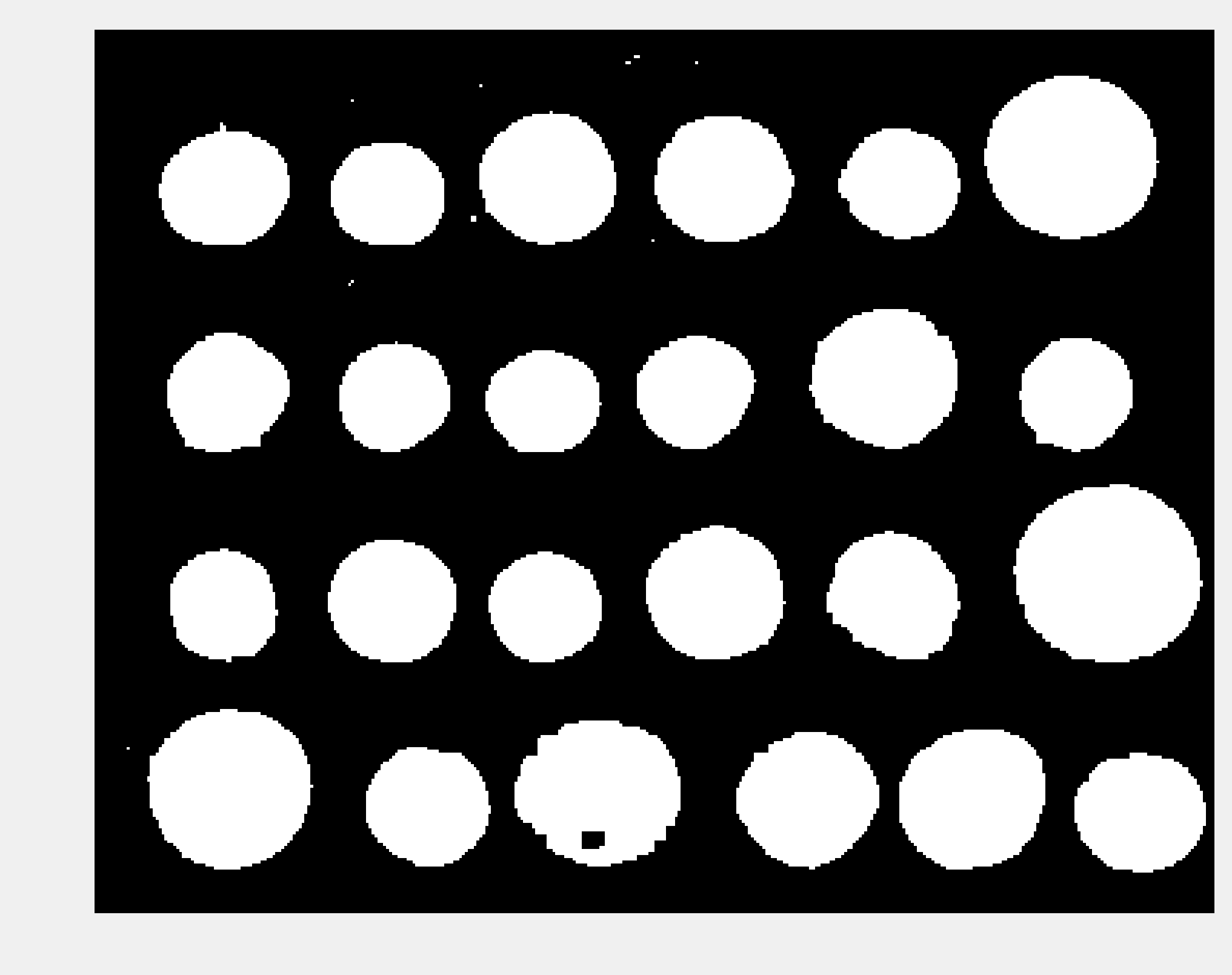
6. The threshold 120 looks better. The next step consists of cleaning the binary image by smoothing the coins and removing the border. scikit-image contains a few functions for these purposes.
img_bin = clear_border(closing(img > 120, square(5)))
show(img_bin)
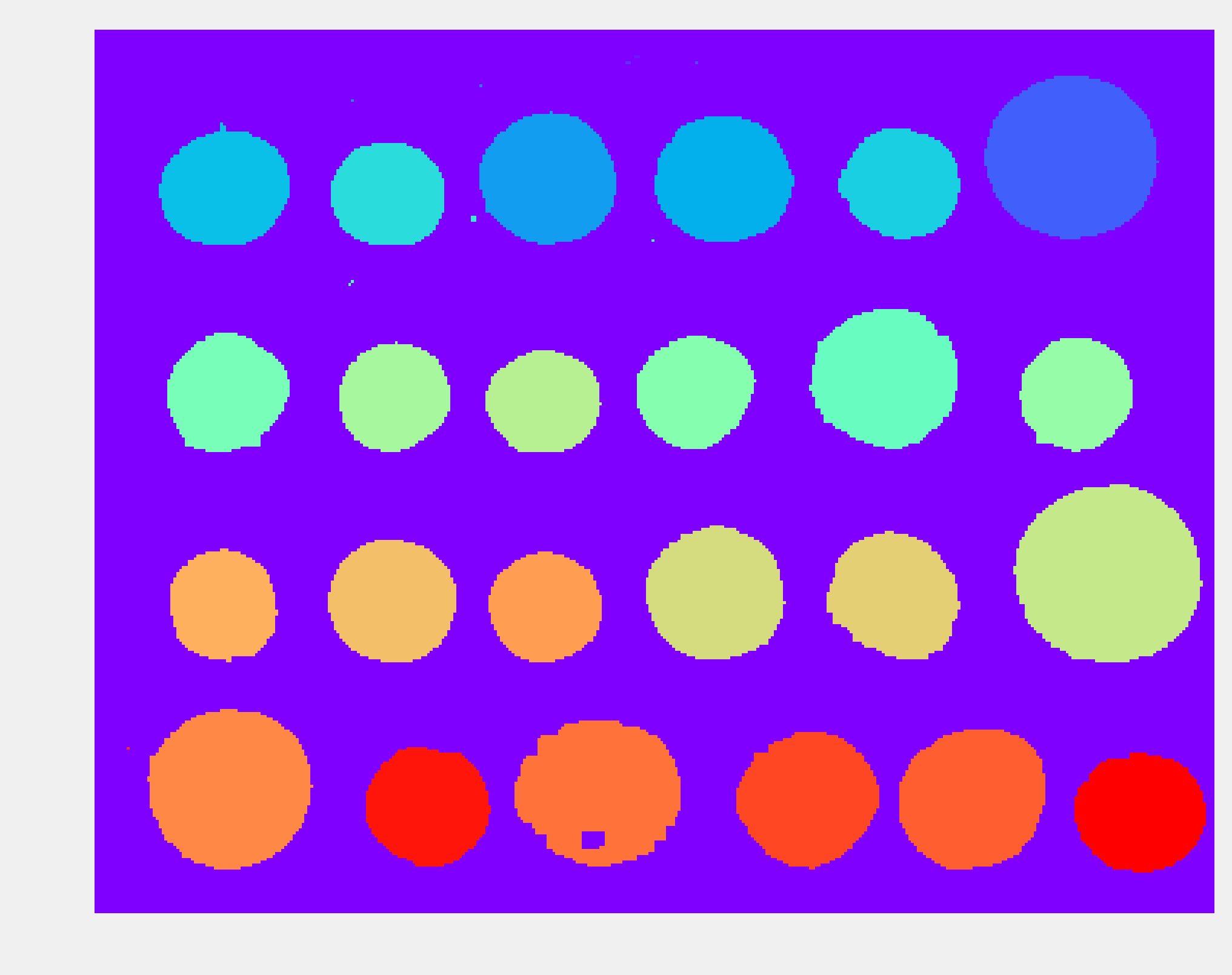
7. Next, we perform the segmentation task itself with the label() function. This function detects the connected components in the image and attributes a unique label to every component. Here, we color code the labels in the binary image:
labels = label(img_bin)
show(labels, cmap=plt.cm.rainbow)
8. Small artifacts in the image result in spurious labels that do not correspond to coins. Therefore, we only keep components with more than 100 pixels. The regionprops() function allows us to retrieve specific properties of the components (here, the area and the bounding box):
regions = regionprops(labels)
boxes = np.array([label['BoundingBox']
                  for label in regions
                  if label['Area'] > 100])
print(f"There are {len(boxes)} coins.")
There are 24 coins.
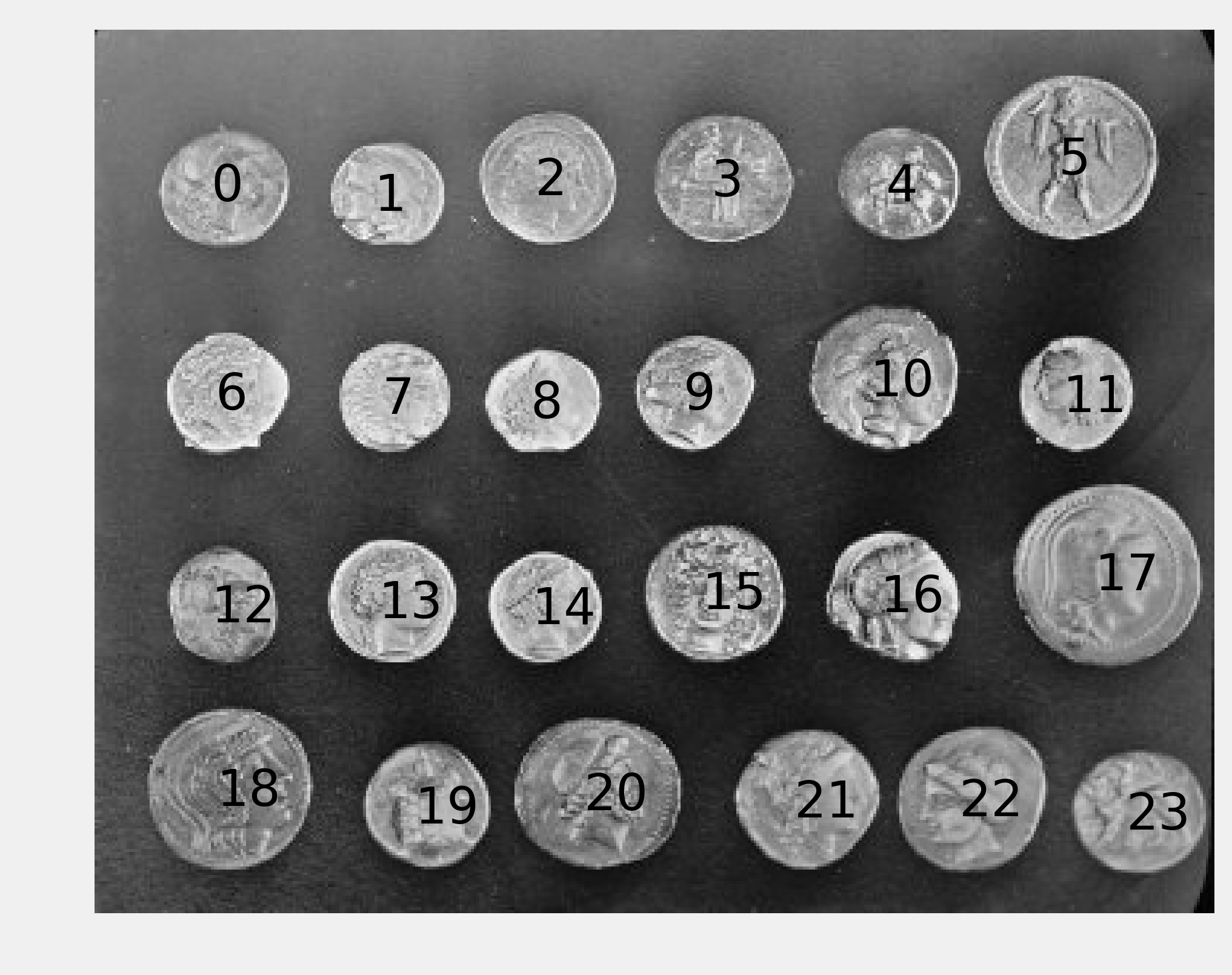
9. Finally, we show the label number on top of each component in the original image:
fig, ax = plt.subplots(1, 1, figsize=(8, 6))
ax.imshow(img, cmap=plt.cm.gray)
ax.set_axis_off()

# Get the coordinates of the boxes.
xs = boxes[:, [1, 3]].mean(axis=1)
ys = boxes[:, [0, 2]].mean(axis=1)

# We reorder the boxes by increasing
# column first, and row second.
for row in range(4):
    # We select the coins in each of the four rows.
    if row < 3:
        ind = ((ys[6 * row] <= ys) &
               (ys < ys[6 * row + 6]))
    else:
        ind = (ys[6 * row] <= ys)
    # We reorder by increasing x coordinate.
    ind = np.nonzero(ind)[0]
    reordered = ind[np.argsort(xs[ind])]
    xs_row = xs[reordered]
    ys_row = ys[reordered]
    # We display the coin number.
    for col in range(6):
        n = 6 * row + col
        ax.text(xs_row[col] - 5, ys_row[col] + 5,
                str(n),
                fontsize=20)
How it works...
To clean up the coins in the thresholded image, we used mathematical morphology techniques. These methods, based on set theory, geometry, and topology, allow us to manipulate shapes.
For example, let's explain dilation and erosion. First, if \(A\) is a set of pixels in an image, and \(b\) is a 2D vector, we denote \(A_b\) the set \(A\) translated by \(b\) as:
Let \(B\) be a set of vectors with integer components. We call B the structuring element (here, we used a square). This set represents the neighborhood of a pixel. The dilation of \(A\) by \(B\) is:
The erosion of \(A\) by \(B\) is:
A dilation extends a set by adding pixels close to its boundaries. An erosion removes the pixels of the set that are too close to the boundaries. The closing of a set is a dilation followed by an erosion. This operation can remove small dark spots and connect small bright cracks. In this recipe, we used a square structuring element.
There's more...
Here are a few references:
- SciPy lecture notes on image processing available at http://scipy-lectures.github.io/packages/scikit-image/
- Image segmentation on Wikipedia, available at https://en.wikipedia.org/wiki/Image_segmentation
- Otsu's method to find a threshold explained at https://en.wikipedia.org/wiki/Otsu's_method
- Segmentation tutorial with scikit-image (which inspired this recipe) available at http://scikit-image.org/docs/dev/user_guide/tutorial_segmentation.html
- Mathematical morphology on Wikipedia, available at https://en.wikipedia.org/wiki/Mathematical_morphology
- API reference of the skimage.morphology module available at http://scikit-image.org/docs/dev/api/skimage.morphology.html
See also
- Computing connected components in an image, in Chapter 14, Graphs and Geometry chapter.