11.1. Manipulating the exposure of an image
 This is one of the 100+ free recipes of the IPython Cookbook, Second Edition, by Cyrille Rossant, a guide to numerical computing and data science in the Jupyter Notebook. The ebook and printed book are available for purchase at Packt Publishing.
▶ Text on GitHub with a CC-BY-NC-ND license
▶ Code on GitHub with a MIT license
▶ Go to Chapter 11 : Image and Audio Processing
▶ Get the Jupyter notebook
The exposure of an image tells us whether the image is too dark, too light, or balanced. It can be measured with a histogram of the intensity values of all pixels. Improving the exposure of an image is a basic image-editing operation. As we will see in this recipe, it can be done easily with scikit-image.
Getting ready
scikit-image should be included by default in Anaconda. Otherwise, you can always install it manually with conda install scikit-image.
How to do it...
1. Let's import the packages:
import numpy as np
import matplotlib.pyplot as plt
import skimage.exposure as skie
%matplotlib inline
2. We open an image with matplotlib. We only take a single RGB component to have a grayscale image (it is a very crude way of doing it, we give much better ways at the end of this recipe):
img = plt.imread('https://github.com/ipython-books/'
                 'cookbook-2nd-data/blob/master/'
                 'beach.png?raw=true')[..., 0]
3. We create a function that displays the image along with its histogram of the intensity values (that is, the exposure):
def show(img):
    # Display the image.
    fig, (ax1, ax2) = plt.subplots(1, 2,
                                   figsize=(12, 3))

    ax1.imshow(img, cmap=plt.cm.gray)
    ax1.set_axis_off()

    # Display the histogram.
    ax2.hist(img.ravel(), lw=0, bins=256)
    ax2.set_xlim(0, img.max())
    ax2.set_yticks([])

    plt.show()
4. Let's display the image along with its histogram:
show(img)
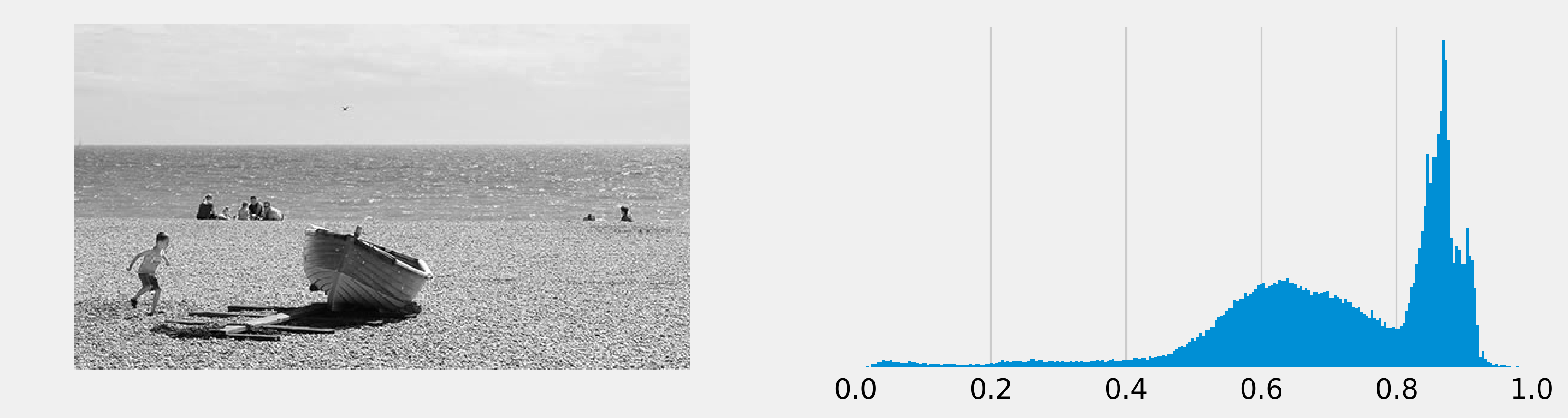
The histogram is unbalanced and the image appears overexposed (many pixels are too bright).
5. Now, we rescale the intensity of the image using scikit-image's rescale_intensity function. The in_range and out_range parameters define a linear mapping from the original image to the modified image. The pixels that are outside in_range are clipped to the extremal values of out_range. Here, the darkest pixels (intensity less than 100) become completely black (0), whereas the brightest pixels (>240) become completely white (255):
show(skie.rescale_intensity(
    img, in_range=(0.4, .95), out_range=(0, 1)))
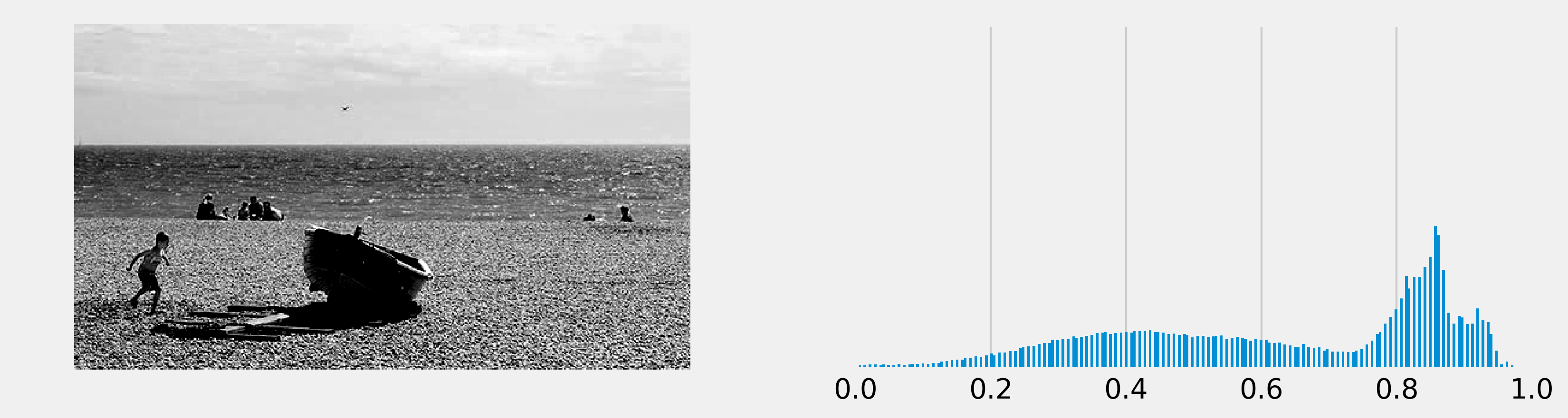
Many intensity values seem to be missing in the histogram, which reflects the poor quality of this crude exposure correction technique.
6. We now use a more advanced exposure correction technique called Contrast Limited Adaptive Histogram Equalization (CLAHE):
show(skie.equalize_adapthist(img))
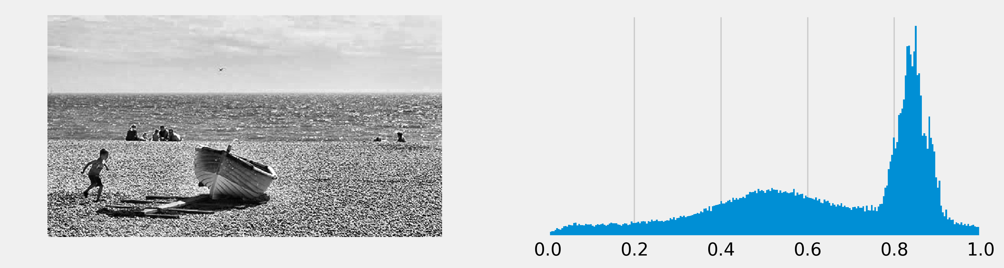
The histogram seems more balanced, and the image now appears more contrasted.
How it works...
An image's histogram represents the distribution of the pixels' intensity values. It is a central tool in image editing, image processing, and computer vision.
The rescale_intensity() function stretches or shrinks the intensity levels of the image. One use case is to ensure that the whole range of values allowed by the data type is used by the image.
The equalize_adapthist() function works by splitting the image into rectangular sections and computing the histogram for each section. Then, the intensity values of the pixels are redistributed to improve the contrast and enhance the details.
The skimage.color.rgb2gray() function converts a colored image to a grayscale image using a special weighting of the color channels that preserves luminance.
There's more...
Here are some references:
- Transforming image data in the scikit-image documentation, at http://scikit-image.org/docs/dev/user_guide/transforming_image_data.html
- Histogram equalization in the scikit-image documentation, at http://scikit-image.org/docs/dev/auto_examples/color_exposure/plot_equalize.html
- Image histogram on Wikipedia, available at https://en.wikipedia.org/wiki/Image_histogram
- Histogram equalization on Wikipedia, available at https://en.wikipedia.org/wiki/Histogram_equalization
- Adaptive histogram equalization on Wikipedia, available at https://en.wikipedia.org/wiki/Adaptive_histogram_equalization
- Contrast on Wikipedia, available at https://en.wikipedia.org/wiki/Contrast_(vision)
See also
- Applying filters on an image